User Guide: How to create a FEMMT model

This guide explains how a model can be created in femmt and provides all the necessary information to work with femmt. Many examples for femmt models can be found in the example folder.

Working directory

Every femmt model has a working directory which can be set when creating an instance of the femmt base class called MagneticComponent. When running the simulation many files will be created in the working directory including the model, mesh and multiple result files. It also contains the electro_magnetic_log.json which the most important simulation results (e.g. losses, inductance, …).

Besides the working directory a MagneticComponent also needs a ComponentType. Currently this can be ‘Inductor’, ‘Transformer’ or ‘IntegratedTransformer’.

This results to the following code:

import femmt as fmt

geo = fmt.MagneticComponent(simulation_type=fmt.SimulationType.FreqDomain,
                             component_type=fmt.ComponentType.Transformer, working_directory=working_directory,
                             verbosity=fmt.Verbosity.ToConsole, is_gui=is_test)

The simulation_type specifies the type of simulation to be performed.

• If set to FreqDomain, indicating a frequency domain simulation.

• If set to TimeDomain, indicating a time domain simulations.

The Verbosity controls the level of detail in the output.

• If set to ToConsole, all output messages are shown in the commend line .

• If set to ToFile, all output messages are written to files.

• If set to Silent, no command line outputs are shown.

This simple feature significantly speeds up simulation time, especially for many automated simulations.

Creating a core

In general, only 2D rotationally symmetric geometries are represented in FEMMT. Other core shapes must first be converted to a 2D rotationally symmetric shape. The corresponding values for this (diameter core, dimensions of the winding window) are taken from the data sheet. Afterwards, a corresponding geometry is generated automatically.

The following graphics always show only a sectional view of the core geometry.

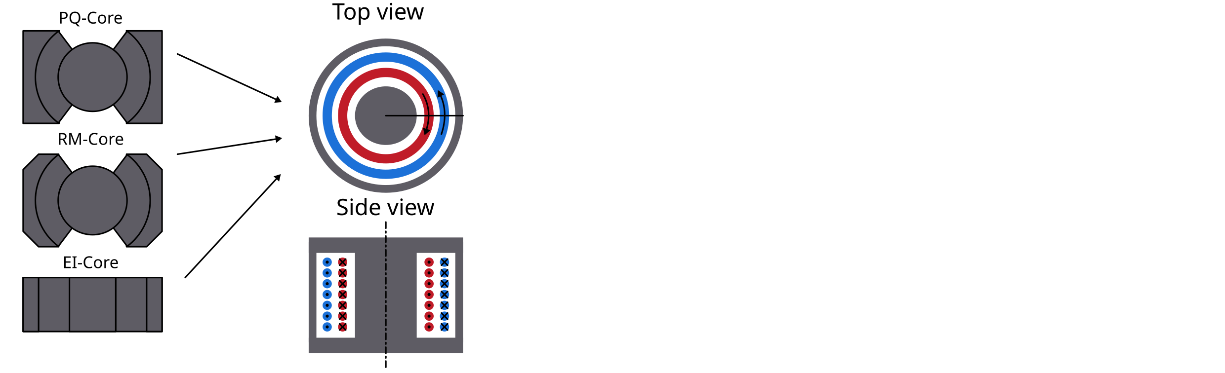
After creating a MagneticComponent, a core needs to be created. The core needs spatial parameters as well as material parameters. The neccessary spatial parameters are shown in the image below.

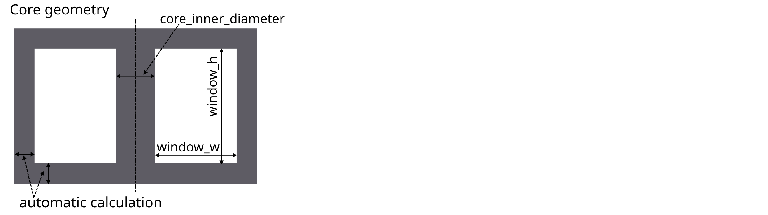
Core spatial parameters can be entered manually but FEMMT provides a database of different practical cores. This database can be accessed using:

core_db = fmt.core_database()["PQ 40/40"]

Now the core object can be created and added to the model (geo object)

core_dimensions = fmt.dtos.SingleCoreDimensions(core_inner_diameter=core_db["core_inner_diameter"],
                                                 window_w=core_db["window_w"],
                                                 window_h=core_db["window_h"],
                                                 core_h=core_db["core_h"])

core = fmt.Core(core_type=fmt.CoreType.Single,
                 core_dimensions=core_dimensions,
                 detailed_core_model=False,
                 material=mdb.Material.N49, temperature=45, frequency=inductor_frequency,
                 permeability_datasource=fmt.MaterialDataSource.Measurement,
                 permeability_datatype=fmt.MeasurementDataType.ComplexPermeability,
                 permeability_measurement_setup=mdb.MeasurementSetup.LEA_LK,
                 permittivity_datasource=fmt.MaterialDataSource.Measurement,
                 permittivity_datatype=fmt.MeasurementDataType.ComplexPermittivity,
                 permittivity_measurement_setup=mdb.MeasurementSetup.LEA_LK, mdb_verbosity=fmt.Verbosity.Silent)
geo.set_core(core)

Material database

The material database was already introduced in the upper code example with the material= parameter. The temperature as well as the frequency are necessary to pick the corresponding data from the datasheet.

Adding air gaps to the core

In the next steps air gaps can be added. Currently it is only possible to add air gaps in the center leg, there for the ‘AirGapLegPosition’ is always ‘CenterLeg’. To set the vertical position for a air gap multiple methods are available:

• Center: The air gap will always be positioned in the center

• Percent: A value between 0 and 100 can be given. Where 0 represents the bottom end and 100 the top end of the winding window.

• Manually: The specific y-coordinate needs to be entered manually.

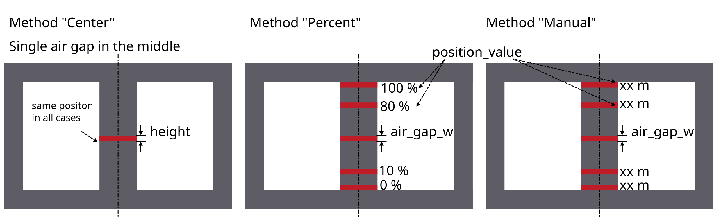
Have a look at the following example on how to create an air gap object and add it to the model:

air_gaps = fmt.AirGaps(method=fmt.AirGapMethod.Percent, core=core)
air_gaps.add_air_gap(leg_position=fmt.AirGapLegPosition.CenterLeg, height=0.0005, position_value=50)
geo.set_air_gaps(air_gaps)

Adding an air_gap object is not necessary. If no air gap is needed, don’t add the air gap object to the model.

Set insulation distances

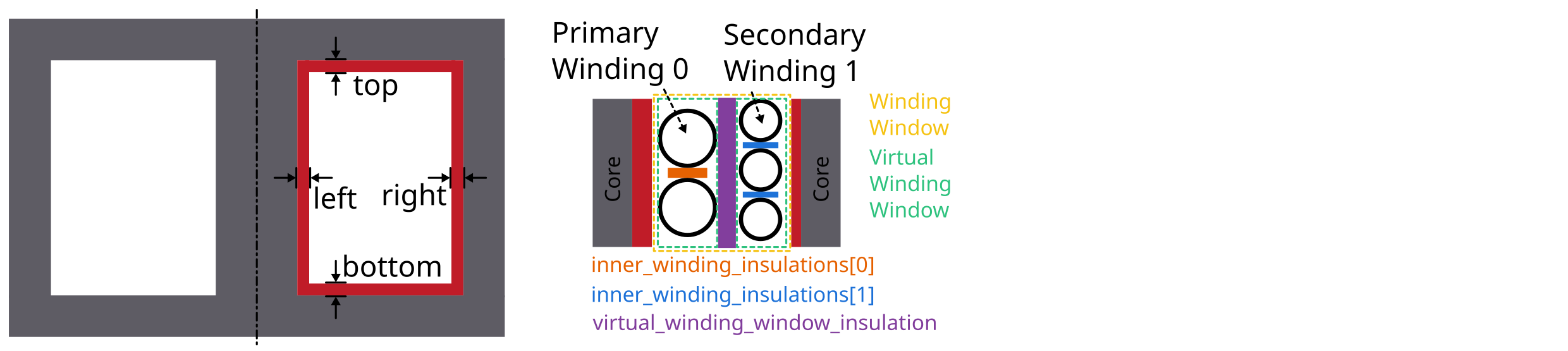
There are multiple insulations implemented in femmt. Some of them are created as rectangles in the model, some are just adding an offset to the windings.

Core insulations are the insulations which are created as rectangles in the model. 4 core insulations will be added: top, bottom, left, right. The distance of those values can be set with the add_core_insulations function. The order of add_core_insulations is as follow : top, bottom, left, and right.

Furthermore there are offset insulations between each turn in the same winding, a distance between 2 windings in one virtual winding window and a distance between each virtual winding window. The first two are set using the add_winding_insulations functions, the last one when creating such a Virtual Winding Windows (vww) .

The add_winding_insulations contains the inner winding insulation, which is a nested lists representing the insulations between turns of the same winding. Importantly, these values are not arranged according to the sequence in which conductors are added to each winding. Instead, the organization is based on the winding number with conductors sorted in ascending order of these numbers. Thus, the first sublist (index 0) corresponds to the winding with the lowest number, the second sublist (index 1) to the winding with the next lowest number, and so on.

This is how to create an insulation object and add certain insulations:

insulation = fmt.Insulation(flag_insulation=True)
insulation.add_core_insulations(0.001, 0.001, 0.002, 0.001)
insulation.add_winding_insulations([[0.0002, 0.001],[0.001, 0.0002]])
geo.set_insulation(insulation)

The spatial parameters for the insulation, as well as for every other function in FEMMT, are always in SI-Units, in this case metres.

Add windings to the winding window

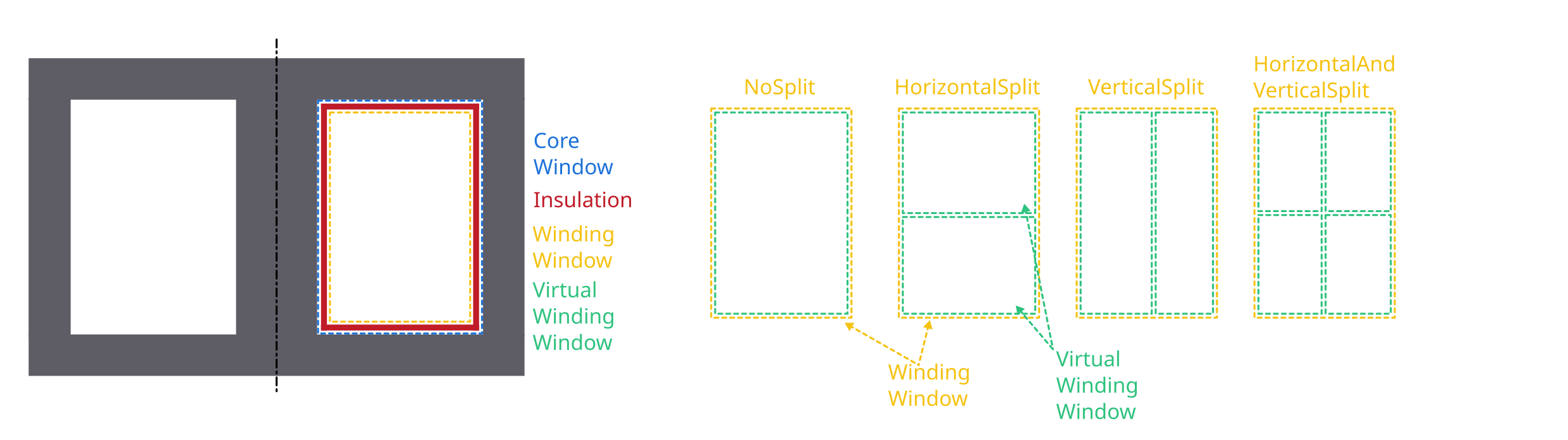
In order to understand the way winding windows work in femmt, the concept of virtual winding windows must be explained:

Virtual Winding Windows

For every femmt model there is always one winding window, which is a 2D representation of the 3D rotated winding window. This winding window can be split into multiple virtual winding windows which are used to draw the conductors. The split_window function has multiple ways to split a winding window into:

• NoSplit: Only 1 virtual winding window will be returned and it has the same size as the real winding window.

• HorizontalSplit: 2 virtual winding windows will be returned, one for the top and one for the bottom part. The height of the splitting line can be set using a horizontal_split_factor (value between 0 and 1)

• VerticalSplit: 2 virtual winding windows will be returned, one for the left and one for the right part. The radius (x-coordinate) of the splitting line can be set using a vertical_split_factor (value between 0 and 1)

• HorizontalAndVerticalSplit: 4 virtual winding windows are returned. One for each corner (in the following order): top_left, top_right, bottom_left, bottom_right. In this case the horizontal and vertical split factors can be used to set the sizes of each grid cell.

In addition to that 2 virtual winding windows can be combined to one (this is not possible for (top_left, bottom_right) or (top_right, bottom_left) combinations). This is done using the combine_vww() function of the WindingWindow class.

Each virtual winding window can be filled with either one single winding or one interleaved winding.

A winding window with only one virtual winding window can be craeted like this:

winding_window = fmt.WindingWindow(core, insulation)
vww = winding_window.split_window(fmt.WindingWindowSplit.NoSplit)

Additionally, the NCellsSplit function provides even more flexibility, allowing the winding window to be split into N columns horizontally. The distance between the virtual winding windows, horizontal split factors, and the vertical split factor can be specified. A winding window with 12 columns horizontally can be created like this:

winding_window = fmt.WindingWindow(core, insulation)
cells = winding_window.NCellsSplit(0, [1 / 6, 2 / 6, 3 / 6, 4 / 6, 5 / 6], 0.5)

Furthermore, the NHorizontalAndVerticalSplit function introduces more advanced splitting capabilities by allowing the winding window to be split into N columns horizontally,with each having M_N rows (vertically). Users can specify the positions of borders between columns and rows to customize the layout of the resulting virtual winding windows. Creating a winding window with three columns, where the second column is further divided into three rows, can be achieved with the following code:

winding_window = fmt.WindingWindow(core, insulation)
cells = winding_window.NHorizontalAndVerticalSplit(horizontal_split_factors=[0.48, 0.75],
                                                  vertical_split_factors=[None, [0.5, 0.85], None])

Winding types and winding schemes

The following table gives an overview of the different winding types, winding schemes and conductor arrangements:

WindingType	ConductorType	WindingScheme	ConductorArrangement	WrapParaType	status	description
Interleaved						Always needs 2 conductors
	RoundSolid, RoundLitz
		Bifilar			not implemented	TODO
		VerticalAlternating			not implemented	primary and secondary winding are interleaved vertically (rows)
		HorizontalAlternating			implemented	primary and secondary winding are interleaved horizontally (cols)
		VerticalStacked			implemented	primary winding is drawn bottom to top, seoncdary winmding is drawn top to bottom
			Square		“
			Hexagonal		“
	RectangularSolid				not implemented
Single						Always needs 1 conductor
	RoundSolid, RoundLitz
		None			implemented
			Square		“
			Square full width		“
			Hexagonal		“
	RectangularSolid
		Full			implemented	whole virtual winding window contains is filled with one turn
		FoilHorizontal (stacked)			implemented	foils are very long (x-axis) and drawn along y-axis
		Square full width			not implemented	foils are drawn along x-axis first and then along y-axis
		FoilVertical			implemented	foils are very tall (y-axis) and drawn along x-axis
				Fixed Thickness	“
				Interpolate	“

ConductorArrangement

• Square: conductors are set in next to each other in a grid

• Hexagonal: similar to square but in this case the conductors frpmo the next column slips in the free space between two conductors from the first column

• Square full width: conducors are first drawn along x-axis and then y-axis

WrapParaType

• Fixed thickness: TODO

• Interpolate: TODO

Images for the possible winding types can be found here.

Add conductors

When creating an instance of the class Conductor a winding number and a conductivity needs to be given:

The winding number represents the index of the winding (e.g. primary->1, secondary->2, tertiary->3). As an example: When starting a simulation on a transformer a current needs to be given, this is done in a list. The first index of the current’s list will be set to the winding with the lowest winding number, the second index of the list to the winding with the second lowest winding number and so on.

The conductivity can be set using the Conductivity enum where one of two possible materials need to be selected:

• Copper

• Aluminium

After creating an conductor object it is necessary to add a conductor to it. As already shown in the winding types table 3 different conducors can be set:

• RoundSolid

• RoundLitz

• RectangularSolid

To create a conductor have a look at the following code example:

winding1 = fmt.Conductor(winding_number=0, conductivity=fmt.Conductivity.Copper)
winding1.set_solid_round_conductor(conductor_radius=0.0011, conductor_arrangement=fmt.ConductorArrangement.Square)

Add conductors to virtual winding windows

Now the conductors need to be added to the virtual winding windows with the corresponding winding type and winding scheme. In this case the set_winding() or set_interleaved_winding() function needs to be called. In the set_interleaved_winding() function an insulation distance can also be set. This value represents the distance between conductors from the primary and secondary side.

vww.set_winding(winding, 14, None, fmt.Align.ToEdges, placing_strategy=fmt.ConductorDistribution.VerticalUpward_HorizontalRightward, zigzag=False)

If you have a look at the winding types and winding schemes table a winding scheme is not needed when creating a round solid conductor in single winding. Therefore the value is set to None.

In the configuration of single windings using round solid or litz wire conductors, the focus is on two main aspects: alignment and how the conductors are placed.

Alignment

Alignment pertains to how the set of conductors is positioned within the winding window:

• Align.ToEdges: Ensures the outermost conductors are close to the winding window’s edges.

• Align.CenterOnHorizontalAxis: Center the winding along the window’s horizontal axis, for balanced distribution.

• Align.CenterOnVerticalAxis: Center the winding along the window’s vertical axis, for balanced distribution.

Placement Strategies

The strategy for placing conductors is named based on the initial direction and subsequent movement. It is only applied if the winding type is Single.

For RoundSolid and RoundLitz conductors, the placement strategies are as follows:

• VerticalUpward_HorizontalRightward: Placement starts at the bottom, moving upward vertically, then shifts rightward horizontally for the next column.

• VerticalUpward_HorizontalLeftward: Placement starts at the bottom, moving upward vertically, then shifts leftward horizontally for the next column.

• VerticalDownward_HorizontalRightward: Begins placement from the top, moving downward, with a rightward shift for each new column.

• VerticalDownward_HorizontalLeftward: Begins placement from the top, moving downward, with a leftward shift for each new column.

• HorizontalRightward_VerticalUpward: Starts on the left side, moving rightward, then upward for each new row.

• HorizontalRightward_VerticalDownward: Starts on the left side, moving rightward, then downward for each new row.

• HorizontalLeftward_VerticalUpward: Starts on the right side, moving leftward, then upward for each new row.

• HorizontalLeftward_VerticalDownward: Starts on the right side, moving leftward, then downward for each new row.

For RectangularSolid conductors, where the winding scheme is FoilVertical or FoilHorizontal, the placement strategies are as follows:

• FoilVerticalDistribution: These strategies are used when distributing rectangular foil conductors vertically.

  • HorizontalRightward: Begins placement from the left of the winding window, moving horizontally rightward for each conductor.

  • HorizontalLeftward: Begins placement from the right of the winding window, moving horizontally leftward for each conductor.

• FoilHorizontalDistribution: These strategies are used when distributing rectangular foil conductors horizontally.

  • VerticalUpward: Begins placement from the bottom of the winding window, moving upward for each conductor.

  • VerticalDownward: Begins placement from the top of the winding window, moving downward for each conductor.

Zigzag Condition

Zigzag placement introduces an alternating pattern in the layout:

• After completing a row or column, the direction alternates (e.g., if moving upward initially, the next is downward).

• The zigzag parameter is optional and defaults to False. It can be omitted if a zigzag movement is not needed.

It can only be used for RoundSolid and RoundLitz conductors when the winding type is Single.

Before the simulation, the winding window must be added to the model:

geo.set_winding_windows([winding_window])

Create model and start simulation

After every needed component is added to the model the model can be created. This is done using the create_model() function. The frequency is needed there because of the mesh which is adapted according to the skin depth. In addition to that a boolean can be given to show the model after creation (in gmsh).

The last step is to run a simulation using single_simulation() or time_domain_simulation depending on the simulation type, where every type needs the following parameters:

For Frequency Domain Simulation: the frequency, currents (and phase if transformer is set) are needed as parameters.

geo.create_model(freq=inductor_frequency, pre_visualize_geometry=show_visual_outputs, save_png=False)
geo.single_simulation(freq=inductor_frequency, current=[4.5],
                      plot_interpolation=False,
                      show_fem_simulation_results=show_visual_outputs)

For Time Domain Simulation: the current_period_vec , time_period_vec ,and number_of_periods are needed as parameters. Users can generate the current_period_vec by creating nested lists, adjusting the structure based on the number of windings. The time_period_vec parameter corresponds to a list of time values associated with the simulation. Additionally, number_of_periods specifies the total number of periods to be simulated. The current_period_vec as The show_rolling_average parameter is a boolean flag that determines whether to display or hide the rolling average of simulation results during the time domain simulation.

geo.create_model(freq=inductor_frequency, pre_visualize_geometry=show_visual_outputs, save_png=False)
geo.time_domain_simulation(current_period_vec=[[0, 1, 0, -1, 0 ], [0, 1, 0, -1, 0]]
                           time_period_vec=[0, 0.1, 0.2, 0.3, 0.4]
                           number_of_periods=2,
                           plot_interpolation=False,
                           show_fem_simulation_results=True,
                           show_rolling_average=False,                                rolling_avg_window_size=50)

Note

Gmsh windows open at various points in the simulations, e.g. to display the geometry or simulation results. To continue (e.g. to start the simulation from the geometry view), simply close the window.

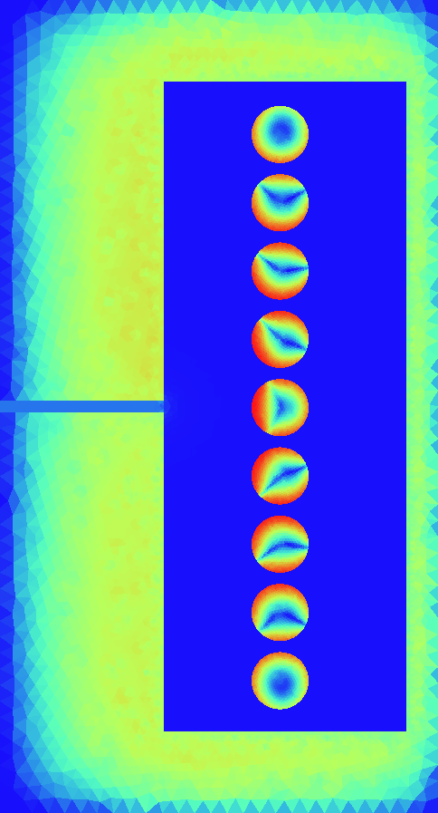
The results should look like this:

Mesh Customization

Understanding and modifying the mesh in FEMMT is crucial for optimizing simulation performance and accuracy. Below are some practical hints to manually adapt the mesh using the meshing factors for different parts of the model, such as the core, winding windows (ww), and air gaps.

Conductor meshing

In general, there are two different approaches to mesh wires:

• for solid conductors, the mesh is adapted according to the skin depth, depending on the frequency. In a frequency sweep, the mesh is generated for the highest frequency.

• for litz conductors, there is a rough mesh only. There is a pre- and postprocessing according to the following papers:

  • Niyomsatian, Korawich and Gyselinck, Johan. and Sabariego, Ruth V.: New closed-form proximity-effect complex permeability expression for characterizing litz-wire windings

  • Niyomsatian, K and Van den Keybus, J. and Sabariego, R. V. and Gyselinck, J.: Frequency-domain homogenization for litz-wire bundles in finite element calculations

Manually Adapting the Mesh

To manually adapt the mesh, the user can adjust the mesh accuracy settings directly in FEMMT setup. These settings control the density of the mesh around different components of the model:

• Mesh Accuracy Core: It affects the density of the mesh around the magnetic core. Decreasing this value increases the mesh density, which can enhance accuracy at the cost of increased computational time.

• Mesh Accuracy Window: It controls the mesh density around the winding window.

• Mesh Accuracy Conductor: It controls the mesh density of the conductors in the winding window. Higher accuracy ensures better representation of conductor shapes and edges.

• Mesh Accuracy Air Gaps: It determines the mesh granularity in the air gaps, which can be important for capturing the magnetic field distribution accurately.

Here’s how the user can customize the mesh accuracies for different components of the magnetic model in Component.py file:

padding = 1.5  # mesh boundary around the model
mu_0 = 4e-7 * np.pi  # vacuum permeability
self.mesh_data = MeshData(mesh_accuracy_core=0.5,
                          mesh_accuracy_window=0.5,
                          mesh_accuracy_conductor=0.5,
                          mesh_accuracy_air_gaps=0.5,
                          padding=padding,
                          mu0=mu_0)

Viewing the Mesh in Gmsh

To visualize the mesh in Gmsh after it has been generated, there are two ways to view the mesh:

Option 1: Direct Visualization in Gmsh

1. Open the generated model file (.msh) in Gmsh.

2. Navigate to the Mesh tab in the top menu and select View mesh.

3. Use the mouse wheel to zoom in and out for a detailed view of the mesh.

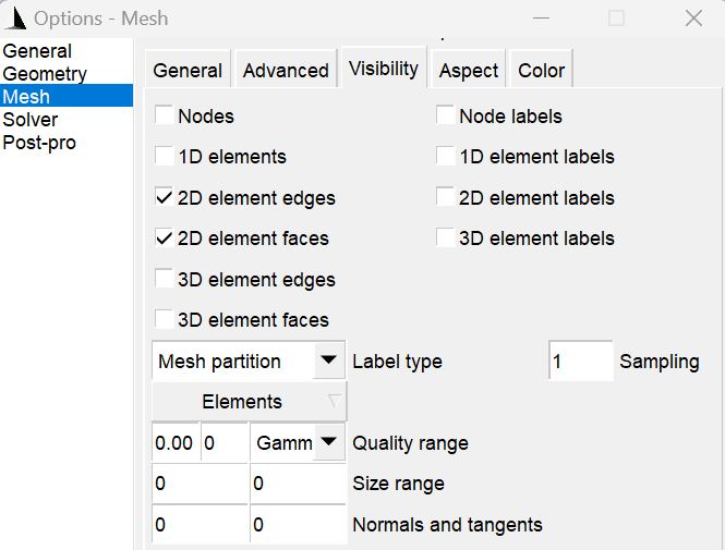
The options panel allows users to control the visibility and labeling of these different element types within the meshing software gmsh as shown in the figure.

Option 2: From the Output Simulation File

For visualizing mesh details from the output simulation file:

1. Double right-click to open the viewing options.

2. Navigate to View -> Visibility -> Mesh Options.

3. Select 2D Element Edges to view the edges of the 2D elements.

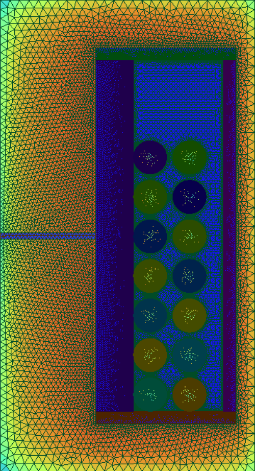
Both options provide insights into how well the different model parts are meshed, which is crucial for ensuring the accuracy of simulation results. The figure below shows the mesh direct from the simulation output of an inductor.

[Optional] Create thermal simulation

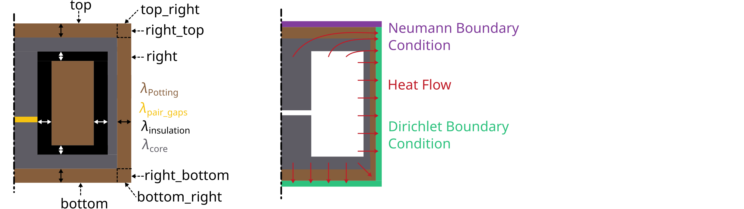
After running the electromagnetic simulation it is possible to use the simulation results and the created model and start a thermal simulation. The thermal simulation will add a case surrounding the previous created model. At the edge of this case the boundary condition is applied and the thermal conductivity as well as the dimensions of the case can be choosen freely. This case is split into 5 parts: top, top right, right, bot right, bot. For each region a different thermal conductivity and boundary condition can be set. In order to run thermal a thermal simulation different values are needed:

• thermal conductivity dict: A dictionary containing thermal conductivities for each region. The regions are: air, core, winding, air_gaps, insulation, case (which is split in top, top_right, right, bot_right, bot

• case gap values: Set the size of the surrounding case

• boundary temperatures dict: The temperatures which will be applied at the edge of the case (dirichlet boundary condition)

• boundary flags: By disabling a specific boundary its condition can be set to a neumann boundary condition ignoring the temperature parameter

Have a look at this example on how to set the parameters since the dictionary keywords are important to write correctly:

thermal_conductivity_dict = {
        "air": 0.0263,
        "case": {
            "top": 0.122,
            "top_right": 0.122,
            "right": 0.122,
            "bot_right": 0.122,
            "bot": 0.122
        },
        "core": 5,
        "winding": 400,
        "air_gaps": 180,
        "insulation": 0.42 if flag_insulation else None
}

case_gap_top = 0.002
case_gap_right = 0.0025
case_gap_bot = 0.002

boundary_temperatures = {
    "value_boundary_top": 20,
    "value_boundary_top_right": 20,
    "value_boundary_right_top": 20,
    "value_boundary_right": 20,
    "value_boundary_right_bottom": 20,
    "value_boundary_bottom_right": 20,
    "value_boundary_bottom": 20
}

boundary_flags = {
    "flag_boundary_top": 0,
    "flag_boundary_top_right": 0,
    "flag_boundary_right_top": 1,
    "flag_boundary_right": 1,
    "flag_boundary_right_bottom": 1,
    "flag_boundary_bottom_right": 1,
    "flag_boundary_bottom": 1
}

In the boundary_flags dictionary 2 flags are set to 0 which means there will be a neumann boundary applied. Please have a look at the picture above which shows the current selected boundaries.

In the following table a possible set of thermal conductivities can be found:

Material	Thermal conductivity
air (background)	0.0263
epoxy resign (used in case)	1.54
ferrite (core)	5
copper (winding)	400
aluminiumnitride (air gaps)	180
polyethylen (insulation)	0.42

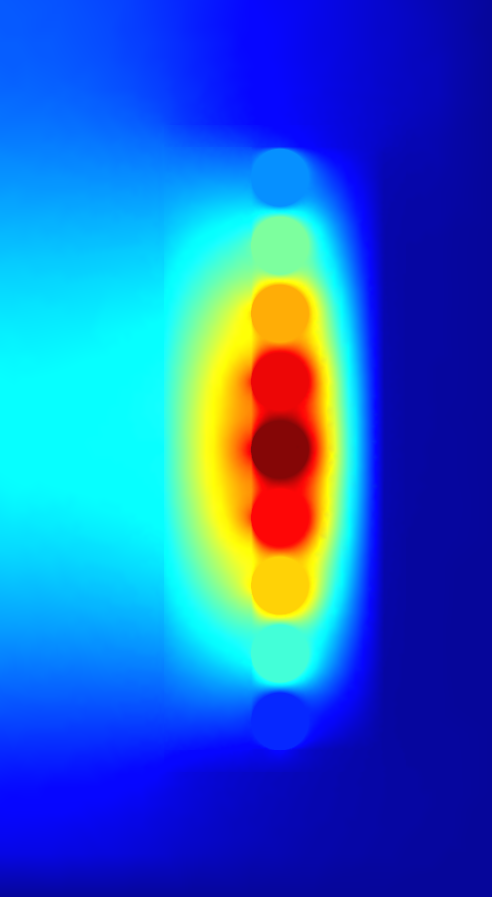
The thermal simulation will solve the stationary heat equation and since no convection is considered every material is assumed to be solid. Now the simulation can be run:

geo.thermal_simulation(thermal_conductivity_dict, boundary_temperatures, boundary_flags, case_gap_top,
                            case_gap_right, case_gap_bot, show_thermal_visual_outputs,
                            color_scheme=fmt.colors_ba_jonas, colors_geometry=fmt.colors_geometry_ba_jonas,
                            flag_insulation=flag_insulation)

The following image shows the simulation results:

How to Read the Result Log

After completing a simulation, the simulation results folder can be found in working_directory/results/. Inside this folder results, the user can find the log_electro_magnetic.json and results_thermal.json files.

• results/log_electro_magnetic.json: This file provides comprehensive details on the electromagnetic aspects of the simulation. It includes information on magnetic flux, currents, voltages, losses, and other key electromagnetic parameters, facilitating a deep understanding of the electromagnetic performance of the simulated system.

• results/results_thermal.json: This file encapsulates the outcomes of thermal analysis, presenting details on the temperatures observed across core components, windings, and insulation materials. It quantifies the minimum, maximum, and mean temperatures for each identified section, offering a comprehensive view of thermal results.

Following table gives an overview over the units of the parameters:

Name:	Frequency	Power Loss	Magnetic Flux	Voltage	Current	Inductance	Resistance
Unit:	Hertz	Watt	Weber	Volt	Ampere	Henry	Ohm

Example Result Log

In this subsection, showcase examples of result logs generated from simulations are shown in two distinct domains: the frequency domain and the time domain. Each domain provides unique insights into the system’s behavior.

Note:

• The values provided in result log are calculated using peak values, not RMS values.

log_electro_magnetic.json File in Frequency Domain

Here is an example of how the outcomes of frequency domain simulation are structured.

{
  "single_sweeps": [
    {
      "f": 200000,
      "winding1": {
        "turn_losses": ["..."],
        "flux": [6.34870443074174e-06, -6.969982393761393e-07],
        "flux_over_current": [3.17434773053773e-06, -3.51948446513906e-07],
        "V": [0.8845429232083418, 7.978006008157411],
        "..."
      },
      "winding2": {
        "..."
      },
      "core_eddy_losses": 0.00050908155779138,
      "core_hyst_losses": 3.16018326710339,
      "core_parts": {
        "core_part_1": {
          "eddy_losses": 0.09956183619015413,
          "hyst_losses": 3.16018326710339,
          "total_core_part_1": 3.259745103293544
        }
      "..."
      "all_winding_losses": 0.5355581006243983
      }
    }
  ],
  "total_losses": {
    "winding1": {
      "total": 0.5355581006244025,
       "turns": ["..."]
    }
    "all_windings": 0.5355581006243983,
    "eddy_core": 0.09956183619015413,
    "hyst_core_fundamental_freq": 3.16018326710339,
    "total_core_part_1": 3.259745103293544,
    "total_eddy_core_part_1": 0.09956183619015413,
    "total_hyst_core_part_1": 3.16018326710339,
    "core": 3.259745103293544,
    "total_losses": 3.7953032039179426
 }
}

Key Components Explained:

• single_sweeps: This array contains data for each frequency sweep performed during the simulation. Each entry in the array represents a set of results for a specific frequency.

  • f: The frequency at which the sweep was conducted.

  • winding1 and winding2: These sections provide detailed results for each winding, including:

    • turn_losses: The power losses (consisting of DC-, Proximity- and Skin-losses) in each turn of the winding.

    • flux: The magnetic flux linked with the winding. The array contains two values, representing the real and imaginary parts of the flux, respectively.

    • flux_over_current: This metric signifies the flux linkage per unit of current and is presented as a complex number, comprising both real and imaginary components.

      • The real part of this value denotes the inductance, reflecting the system’s capacity to store energy within a magnetic field generated by the current through the winding.

      • The imaginary part, initially referred to as “negative resistance”, more aptly relates to the reactive characteristics or the phase shift between the current and magnetic flux linkage.

    • V: Voltage across the winding, with the first value indicating the real part and the second the imaginary part.

    • I: Current through the winding, with similar representation to voltage.

  • core_eddy_losses and core_hyst_losses: These values represent the losses due to eddy currents and hysteresis in the core.

  • core_parts: It provides a detailed breakdown of losses within each segmented part of the core, as the core is divided sometimes into multiple parts. This segmentation is particularly useful for identifying how different sections of the core contribute to the overall eddy current and hysteresis losses, allowing for more targeted improvements in core design and material selection.

    • eddy_losses: Quantifies the losses due to eddy currents for the specific part.

    • hyst_losses: Quantifies the losses due to hysteresis for the specific part.

    • total_core_part_n: The sum of eddy_losses and hyst_losses for the part, providing a total loss figure for that segment.

• total_losses: This section summarizes the overall energy dissipation within the system, combining losses from various components. It is broken down into several key areas:

  • all_windings: It aggregates the losses across all windings in the system.

  • core: This aggregates the losses from all individual segments within the core total_core_part_1, total_core_part_2,.. etc, providing a comprehensive view of the core’s total contribution to the system’s losses.

  • total_losses: it represents the sum of all losses within the system, including windings and core.

log_electro_magnetic.json File in Time Domain

Here is an example of how the outcomes of time domain simulation are structured.

{
  "time_domain_simulation": [
    {
      "f": 100000,
      "T": 1e-05,
      "Timemax": 1.25e-05,
      "number_of_steps": 5,
      "dt": 2.5e-06
    },
    {
      "step_1": {
        "windings": {
          "winding1": {
            "number_turns": 10,
            "flux": [-7.209142581890734e-06],
            "V": [-2.892335944263035],
            "I": 2.0
          },
          "winding2": {
            "..." }}}
    },
    {
     "...": {}
  ],
  "average_losses": {
    "core_eddy_losses": [0.00037330739608363716],
    "core_hyst_losses": [0],
    "winding1": {
      "winding_losses": 1.2578033060966147,
      "flux_over_current": [6.703043813058433e-06],
      "average_current": [0.4],
      "average_voltage": [1.8009901071754213],
      "P": 0.7203960428701686,
      "S": 4.5274565545301515,
      "Q": 4.469775429993662
    },
    "winding2": {"..."}
  },
  "total_losses": {
    "all_windings_losses": 2.511429275334878,
    "eddy_core": 0.00037330739608363716,
    "core": 0.00037330739608363716,
    "total_losses": 2.5118025827309616
  }
}

Key Components Explained:

• time_domain_simulation: An array capturing simulation steps over time, including initial setup and individual time steps.

  • The initial setup specifies the simulation frequency (f), period (T), maximum time (Timemax), total number of steps (number_of_steps), and time increment (dt).

  • step_1 and subsequent steps detail the state of windings at specific times. For example, in step_1, winding1 shows:

    • number_turns: Number of turns in the winding.

    • flux: Magnetic flux through the winding observed in step_1.

    • V: Voltage across the winding observed in step_1.

    • I: Current through the winding observed in step_1.

• average_losses: It captures averaged losses over the simulation period, such as core_eddy_losses, core_hyst_losses, and detailed losses per winding (winding1, winding2). The average current, voltage, active power (P), apparent power (S), and reactive power(Q) are also calculated.

• total_losses: It aggregates all losses within the system, including all_windings_losses, eddy_core losses, and total losses (total_losses), providing a total view of losses.

results_thermal.json File

This section provides an overview and analysis of thermal data, including temperature-related metrics obtained from the electromagnetic simulation. The outcomes of thermal simulation are structured as:

{
  "core_parts": {
    "core_part_1": {
      "min": 20.48340546242281,
      "max": 30.82746116029882,
      "mean": 26.775625696609733
    },
    "total": {
      "min": 20.48340546242281,
      "max": 30.82746116029882,
      "mean": 26.775625696609733
    }
  },
  "windings": {
    "winding_0_0": {"..."},
    "winding_0_1": {"..."},
    "winding_0_2": {"..."},
    "winding_1_0": {"..."},
    "winding_1_1": {"..."},
    "winding_1_2": {"..."},
    "total": {"..."}
  },
  "misc": {
    "case_volume": 0.00017214993340642786,
    "case_weight": -1
  },
  "insulations": {
    "min": 20.57984040880558,
    "max": 34.82921229676766,
    "mean": 27.465726650615863
  }
}

Detailed Overview:

All temperature values mentioned are in degrees Celsius (°C).

• core_parts: This section provides temperature data for different core parts. For instance, for core_part_1:

  • min: Minimum temperature observed.

  • max: Maximum temperature observed.

  • mean: Mean temperature calculated over the simulation.

• total under core_parts aggregates the temperature data for all core parts, providing an overview of the entire core’s thermal behavior.

• windings: The windings section presents temperature data for individual windings, where each winding is identified by a combination of winding number and turn number (e.g., winding_0_0, winding_0_1, etc.). Each winding entry includes:

  • min: Minimum temperature observed.

  • max: Maximum temperature observed.

  • mean: Mean temperature calculated during the simulation.

• total under windings summarizes temperature characteristics across all windings.

• misc: The misc section includes additional thermal information, such as: - case_volume: Volume-related data. - case_weight: Weight-related data.

• insulations: The insulations section provides insights into insulation-related temperature metrics. It includes:

  • min: Minimum insulation temperature observed.

  • max: Maximum insulation temperature observed.

  • mean: Mean insulation temperature calculated over the simulation.

Warnings and Failures

Note

Volumetric mass density not implemented for custom cores. Returns ‘0’ in log-file: Core cost will also result to 0.

As custom cores materials are e.g. ferrite, iron or even a fictive material, calculation with a fixed mass density does not make sense. So, weight (and also core costs) are set to zero in the result log.