1 Scope toolbox for documentation purposes and comparisons

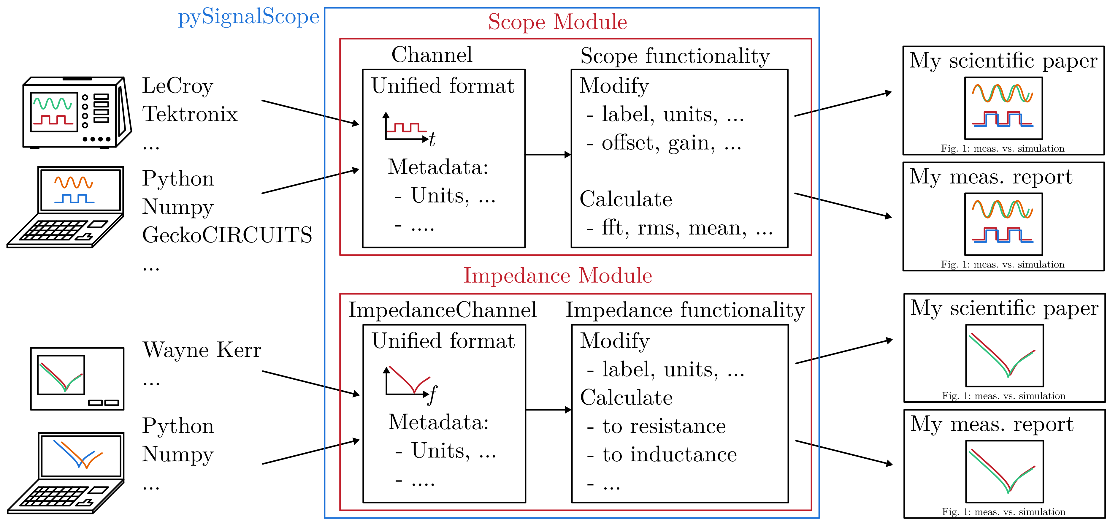
pySignalScope processes and compares time domain data similar to oscilloscopes in electronics. Signals can be filtered, derived, integrated or evaluated. Furthermore, pySignalScope includes a module for evaluating and editing the impedance curves of an impedance analyzer or comparing them with the simulation. The main purpose is the quick and easy evaluation of signals, as well as the targeted generation of images for technical documentation. Some examples are:

Bachelor / Master / Ph.D. theses,
Scientific papers,
Technical manuals, and
Measurement reports.

1.1 Overview

Bring measurements from the oscilloscope and the circuit simulator into a standardized Channel format. Edit the signals by using the Scope functionality: shifting them in time (different zero points) or define the zero point for measuring equipment that can only record AC. Calculate the FFT or important values such as RMS, mean etc. Bring the originally different input formats into common plots to make comparisons easy.

With the Impedance functionality, ImpedanceChannels can be read in, edited and compared. A conversion to e.g. the inductance value is possible with just one command.

https://raw.githubusercontent.com/upb-lea/pySignalScope/main/docs/source/figures/introduction.png

1.2 Getting started

Install this repository into your virtual environment (venv) or jupyter notebook:

pip install pysignalscope

Use the toolbox in your python program:

import pysignalscope as pss
...

1.3 Example usage

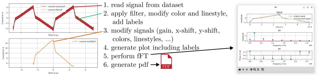
pySignalScope helps to load, edit, display and analyze the signals. The following application example loads a noisy measurement signal, which is first filtered.

import pysignalscope as pss

# Read curves from scope csv file
[voltage_prim, voltage_sec, current_prim, current_sec] = pss.Scope.from_tektronix('scope_example_data_tek.csv')

# Add labels and units to channel: This example considers the Channel 'current_prim' only
current_prim = pss.Scope.modify(current_prim, label='current measured', unit='A', color='red')

# Low pass filter the noisy current signal, modify the Channel attributes label, color and linestyle
current_prim_filtered = pss.Scope.low_pass_filter(current_prim)
current_prim_filtered = pss.Scope.modify(current_prim_filtered, label='current filtered', linestyle='--', color='green')

# Make some modifications on the signal itself: data offset, time offset and factor to the data.
# Short the channel to one period and add label, color and linestyle to the Channel
current_prim_filtered_mod = pss.Scope.modify(current_prim_filtered, data_factor=1.3, data_offset=11, time_shift=2.5e-6)
current_prim_filtered_mod = pss.Scope.short_to_period(current_prim_filtered_mod, f0=200000)
current_prim_filtered_mod = pss.Scope.modify(current_prim_filtered_mod, label='current modified', linestyle='-', color='orange')

# Plot channels, save as pdf
fig1 = pss.Scope.plot_channels([current_prim, current_prim_filtered], [current_prim_filtered_mod], timebase='us')
pss.save_figure(fig1, 'figure.pdf')

# short channels to a single period, perform FFT for current waveforms
current_prim = pss.Scope.short_to_period(current_prim, f0=200000)
current_prim = pss.Scope.modify(current_prim, time_shift=5e-6)
pss.Scope.fft(current_prim)

To simplify the display, colors, linestyle and the label can be attached to the object. This is shown in the plot above.

The lower plot shows the post-processing of the filtered signal. This is multiplied by a small gain, provided with an offset and shortened to a period duration. The label, color and line style are changed. The signals are then plotted with just one plot command.

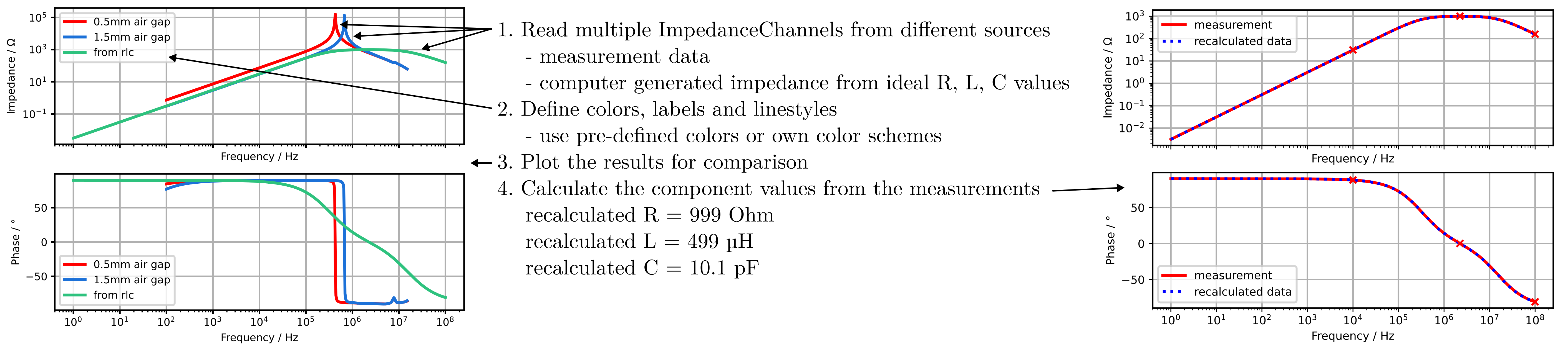
https://raw.githubusercontent.com/upb-lea/pySignalScope/main/docs/source/figures/function_overview.png

The functionality for the Impedance module is similar to the Scope module. In here, ImpedanceChannel objects can be loaded from different sources, which can be a .csv measurement file from an impedance analyzer or a computer generated curve. ImpedanceChannel objects can be modified in attributes and data, plotted and equivalent circuit parameters can be obtained from measurements.

https://raw.githubusercontent.com/upb-lea/pySignalScope/main/docs/source/figures/impedance_function_overview.png

Have a look at the Scope example and at the Impedance example to see what you can do with this toolbox.

1.4 Naming convention

This toolbox is divided into two modules: The functionality of an oscilloscope (Scope) and the functionality of an impedance analyzer (Impedance).

1.4.1 Scope

The Scope module provides functionalities for editing and evaluating individual channels that are also provided by a real oscilloscope - just on a PC. Scope creates, imports, edits or evaluates Channels. The following prefixes apply:

generate_: Generates a new Channel
no prefix: Is applied to a Channel and results in a new Channel (e.g. add() adds two channels)
from_: Generates a Channel from an oscilloscope data set, a simulation program or a calculation (e.g. from_tektronix generates a Channel from a tektronix scope file)
calc_: Calculates individual values from a Channel (e.g. calc_rms() calculates the RMS from a given Channel)
plot_: Plots channels in the desired arrangement (e.g. plot_channels() plots the given Channels)

1.4.2 Impedance

The Impedance module provides functionalities to evaluate impedance curves. Impedance creates, imports, edits or evaluates ImpedanceChannel.

generate_: Generates a new ImpedanceChannel
no prefix: Is applied to a ImpedanceChannel and results in a new ImpedanceChannel (e.g. modify() modifies an ImpedanceChannel)
from_: Generates a ImpedanceChannel from an impedance analyzer data set, a simulation program or a calculation (e.g. from_waynekerr generates a ImpedanceChannel from a real measurement file)
calc_: Calculates individual values from a ImpedanceChannel (e.g. calc_rlc() calculates the equivalent resistance, inductance and capacitance)
plot_: Plots ImpedanceChannel (e.g. plot_impedance() plots the given ImpedanceChannels)

1.5 Documentation

Find the documentation here.

1.6 Bug Reports

Please use the issues report button within GitHub to report bugs.

1.7 Changelog

Find the changelog here.

2 pySignalScope function documentation

Dataclass for Channel objects in a special format, to keep labels, units and voltages belonging to a certain curve.

color: str | Tuple | None: channel color in a plot (optional)

data: array: data series of the channel (mandatory)

label: str | None: channel label displayed in a plot (optional)

linestyle: str | None: channel linestyle in a plot (optional)

source: str | None: channel source, additional meta data (optional)

time: array: time series of the channel (mandatory)

unit: str | None: channel unit displayed in a plot (optional)

class pysignalscope.Scope

Class to share channel figures (multiple in a scope) in a special format, to keep labels, units and voltages belonging to a certain curve.

static add(*channels: Channel) → Channel

Add data of several Channels.

Parameters:: channels (Channel) – Input channels
Returns:: Channel resulting from added input channels
Return type:: Channel

static calc_abs(channel: Channel) → Channel

Modify the existing scope channel so that the signal is rectified.

Parameters:: channel (Channel) – Scope channel object
Returns:: abs(channel.data).
Return type:: Channel

static calc_absmean(channel: Channel) → Any

Calculate the absolute mean of the given channel. Make sure to provide a SINGLE PERIOD of the signal.

Parameters:: channel (Channel) – Scope channel object
Returns:: abs(mean(self.data))
Return type:: Any

static calc_mean(channel: Channel) → Any

Calculate the mean of the given channel. Make sure to provide a SINGLE PERIOD of the signal.

Parameters:: channel (Channel) – Scope channel object
Returns:: mean(self.data)
Return type:: any

static calc_rms(channel: Channel) → Any

Calculate the RMS of a given channel. Make sure to provide a SINGLE PERIOD of the signal.

Parameters:: channel (Channel) – Scope channel object
Returns:: rms(self.data).
Return type:: Any

Graphical comparison for datasets. Note: Datasets need to be type Channel.

Parameters:

channels (Channel) – dataset according to Channel
shift (list[float]) – phase shift in a list for every input dataset (optional parameter)
scale (list[float]) – channel scale factor in a list for every input dataset (optional parameter)
offset (list[float]) – channel offset in a list for every input dataset (optional parameter)
timebase (str) – timebase, can be ‘s’, ‘ms’, ‘us’, ‘ns’ or ‘ps’

static copy(channel: Channel) → Channel

Create a deepcopy of Channel.

Parameters:: channel (Channel) – Scope channel object

static derivative(channel: Channel, order: int = 1) → Channel

Get the derivative of the data.

In case of measured input signal, it is useful to apply a low-pass filter first.

Parameters:

channel (Channel) – Channel object
order (int) – order of derivative with default = 1 (optional parameter) 1 corresponds to 1st order

Returns:

Channel object

Return type:

Channel

static fft(channel: Channel, plot: bool = True)

Perform fft to the signal.

Parameters:

channel (Channel) – Scope channel object
plot (bool) – True (default) to show a figure (optional parameter)

Returns:

numpy-array [[frequency-vector],[amplitude-vector],[phase-vector]]

Return type:

npt.NDArray[list]

Example:

>>> import pysignalscope as pss
>>> import numpy as np
>>> channel_example = pss.Scope.from_numpy(np.array([[0, 5e-3, 10e-3, 15e-3, 20e-3], [1, -1, 1, -1, 1]]), f0=100000, mode='time')
>>> pss.Scope.fft(channel_example)

static from_geckocircuits(txt_datafile: str, f0: float | None = None) → List[Channel]

Convert a gecko simulation file to Channel.

Parameters:

txt_datafile (str) – path to text file, generated by geckoCIRCUITS
f0 (float) – fundamental frequency (optional parameter)

Returns:

List of Channels

Return type:

list[Channel]

static from_lecroy(*csv_files: str) → List[Channel]

Translate LeCroy csv-files to a list of Channel class objects.

Note: insert multiple .csv-files to get a list of all channels

Parameters:: csv_files (str) – csv-file from tektronix scope
Returns:: List of Channel objects
Return type:: List[‘Channel’]
Example single channel:

>>> import pysignalscope as pss
>>> [current_prim] = pss.Scope.from_lecroy('/path/to/lecroy/files/current_prim.csv')

Example multiple channels channel:

>>> import pysignalscope as pss
>>> [current_prim, current_sec] = pss.Scope.from_lecroy('/path/one/current_prim.csv', '/path/two/current_sec.csv')

static from_lecroy_remote(scope_channel_number: int, ip_address: str, label: str) → Channel

Get the data of a LeCroy oscilloscope and return a Channel object with the collected data.

Parameters:

scope_channel_number (int) – number of the channel
ip_address (str) – ip-address of the oscilloscope
label (str) – label name of channel

Returns:

Channel object with collected data

Return type:

‘Channel’

static from_numpy(period_vector_t_i: ndarray, mode: str = 'rad', f0: float | None = None, label: str | None = None, unit: str | None = None) → Channel

Bring a numpy or list array to an instance of Channel.

Parameters:

period_vector_t_i (npt.ArrayLike) – input vector np.array([time], [signal])
mode (str) – ‘rad’ [default], ‘deg’ or ‘time’
f0 (float) – fundamental frequency in Hz (optional parameter)
label (str) – channel label (optional parameter)
unit (str) – channel unit (optional parameter)

Example:

>>> import pysignalscope as pss
>>> import numpy as np
>>> channel = pss.Scope.from_numpy(np.array([[0, 5e-3, 10e-3, 15e-3, 20e-3], [1, -1, 1, -1, 1]]), f0=100000, mode='time')

static from_tektronix(csv_file: str) → List[Channel]

Translate tektronix csv-file to a tuple of Channel.

Note: Returns a tuple with four Channels (Tektronix stores multiple channel data in single .csv-file, this results to return of a tuple containing Channel’s)

Parameters:: csv_file (str) – csv-file from tektronix scope
Returns:: tuple of Channel, depending on the channel count stored in the .csv-file
Return type:: list[Channel, Channel, Channel, Channel]
Example:

>>> import pysignalscope as pss
>>> [voltage, current_prim, current_sec] = pss.Scope.from_tektronix('/path/to/tektronix/file/tek0000.csv')

static from_tektronix_mso58(*csv_files: str) → List[Channel]

Translate tektronix csv-files to a list of Channel class objects.

Note: insert multiple .csv-files to get a list of all channels.

Parameters:: csv_files (str) – csv-file from tektronix scope
Returns:: List of Channel objects
Return type:: List[‘Channel’]
Example single channel:

>>> import pysignalscope as pss
>>> [current_prim] = pss.Scope.from_tektronix_mso58('/path/to/lecroy/files/current_prim.csv')

Example multiple channels channel:

>>> import pysignalscope as pss
>>> [current_prim, current_sec] = pss.Scope.from_tektronix_mso58('/path/one/current_prim.csv', '/path/two/current_sec.csv')

static from_tektronix_mso58_multichannel(csv_file: str) → List[Channel]

Translate tektronix csv-files to a list of Channel class objects.

Note: insert multiple .csv-files to get a list of all channels.

Parameters:: csv_file (str) – csv-file from tektronix scope
Returns:: List of Channel objects
Return type:: List[‘Channel’]
Example multiple channel csv-file:

>>> import pysignalscope as pss
>>> [current_prim, current_sec] = pss.Scope.from_tektronix_mso58_multichannel('/path/to/lecroy/files/currents.csv')

Generate a channel object.

Parameters:

time (List[float] or np.ndarray) – time series
data (List[float] or np.ndarray) – channel data
label (str) – channel label (optional parameter)
unit (str) – channel unit (optional parameter)
color (str or tuple) – channel color (optional parameter)
source (str) – channel source (optional parameter)
linestyle (str) – channel linestyle (optional parameter) e.g.’-’ ‘–’ ‘-.’ ‘:’ see also https://matplotlib.org/stable/gallery/lines_bars_and_markers/linestyles.html

static integrate(channel: Channel, label: str | None = None) → Channel

Integrate a channels signal.

The default use-case is calculating energy loss (variable naming is for the use case to calculate switch energy from power loss curve, e.g. from double-pulse measurement)

Parameters:

channel (Channel) – channel with power
label (str) – channel label (optional parameter)

Returns:

returns a Channel-class, what integrates the input values

Return type:

Channel

static load(filepath: str) → Channel

Load a Channel file from the hard disk.

Parameters:: filepath (str) – filepath
Returns:: loaded Channel object
Return type:: Channel

static low_pass_filter(channel: Channel, order: int = 1, angular_frequency_rad: float = 0.05) → Channel

Implement a butterworth filter on the given signal.

Parameters:

channel (Channel) – Channel object
order (int) – filter order with default = 1 (optional parameter)
angular_frequency_rad (float) – angular frequency in rad. Valid for values 0…1. (optional parameter) with default = 0.05. Smaller value means lower filter frequency.

Returns:

Channel object with filtered data

Return type:

Channel

Modify channel data like metadata or add a factor or offset to channel data.

Useful for classes with time/data, but without labels or units.

Parameters:

channel (Channel) – Scope channel object
data_factor (float) – multiply self.data by data_factor (optional parameter)
data_offset (float) – add an offset to self.data (optional parameter)
label (str) – label to add to the Channel-class (optional parameter)
unit (str) – unit to add to the Channel-class (optional parameter)
color (str or tuple) – Color of a channel (optional parameter)
source (str) – Source of a channel, e.g. ‘GeckoCIRCUITS’, ‘Numpy’, ‘Tektronix-Scope’, … (optional parameter)
time_shift (float) – add time to the time base (optional parameter)
time_shift_rotate (float) – shifts a signal by the given time, but the end of the signal will come to the beginning of the signal. Only recommended for periodic signals! (optional parameter)
time_cut_min (float) – removes all time units smaller than the given one (optional parameter)
time_cut_max (float) – removes all time units bigger than the given one (optional parameter)
linestyle (str) – channel linestyle (optional parameter) for details see parameter description of method ‘generate_channel’

Returns:

Channel object

Return type:

Channel

static multiply(channel_1: Channel, channel_2: Channel, label: str | None = None) → Channel

Multiply two datasets, e.g. to calculate the power from voltage and current.

Parameters:

channel_1 (Channel) – channel_1, e.g. voltage channel
channel_2 (Channel) – channel_2, e.g. current channel
label (str) – label for new dataset_channel (optional parameter)

Returns:

Multiplication of two datasets, e.g. power from voltage and current

Return type:

Channel

static plot_channels(*channel: List[Channel], timebase: str = 's', figure_size: Tuple | None = None, figure_directory: str | None = None) → figure

Plot channel datasets.

Examples:

>>> import pysignalscope as pss
>>> ch1, ch2, ch3, ch4 = pss.Scope.from_tektronix('tektronix_csv_file.csv')
>>> pss.Scope.plot_channels([ch1, ch2, ch3],[ch4])

Plots two subplots. First one has ch1, ch2, ch3, second one has ch4.

Y-axis labels are set according to the unit, presented in the last curve for the subplot. For own axis labeling, use as unit for the last channel your label, e.g. r”$i_T$ in A”. Note, that the r before the string gives the command to accept LaTeX formulas, like $$.

Parameters:

channel (list[Channel]) – list of datasets
timebase (str) – timebase, can be ‘s’, ‘ms’, ‘us’, ‘ns’ or ‘ps’
figure_size (Tuple) – None for auto-fit; fig_size for matplotlib (width, length in mm) (optional parameter)
figure_directory (str) – full path with file extension (optional parameter)

Returns:

Plots

Return type:

None

static plot_shiftchannels(channels: List[Channel], shiftstep_x: float | None = None, shiftstep_y: float | None = None, displayrange_x: Tuple[float, float] | None = None, displayrange_y: Tuple[float, float] | None = None) → list[float]

Plot channel datasets.

Examples:

>>> import pysignalscope as pss
>>> ch1, ch2, ch3, ch4 = pss.Scope.from_tektronix('tektronix_csv_file.csv')
>>> pss.Scope.plot_shiftchannels([ch1, ch2])

Plots the channels ch1 and ch2. You can zoom into by selecting the zoom area with help of left mouse button. By moving the mouse while pressing the button the area is marked by a red rectangle. If you release the left mouse button the area is marked. By moving the mouse within the area an perform a button press, you confirm and you zoom in the area. If you perform the left mouse button click outside of the marked area, you reject the selection. You reject the selection always by clicking the right mouse button independent you zoom out. button. If no area is selected or wait for confirmation, the click on the right mouse button leads to zooming out. There is a zoom limit in both directions. In this case, the rectangle shows the possible area (becomes larger), after you have release the left mouse button.

Y-axis labels are set according to the unit, presented in the last curve for the subplot. For own axis labeling, use as unit for the last channel your label, e.g. r”$i_T$ in A”. Note, that the r before the string gives the command to accept LaTeX formulas, like $$. The parameters has to fullfill conditions: Minimal shift step in x-direction is the minimal difference of 2 points of all provided channels

Parameters:

channels (list[Channel]) – list of datasets
shiftstep_x (float) – shift step in x-direction (optional parameter) Has to be in range ‘minimal difference of 2 points of the channels’ to (‘displayed maximal x-value minus displayed minimal x-value’)/10
shiftstep_y (float) – shift step in y-direction (optional parameter) Has to be in range (‘displayed maximal y-value minus displayed minimal y-value’)/200 to (‘displayed maximal y-value minus displayed minimal y-value’)/10
displayrange_x (tuple of float) – Display range limits in x-direction (min_x, max_x) (optional parameter) Definition: delta_min_x = 100 * ‘minimum distance between 2 samples’, min_x = ‘minimal x-value (of all channels)’, max_x = ‘maximal x-value (of all channels)’, delta_x = max_x-min_x The range for displayrange_x[0]: From min_x-delta_x to max_x-delta_min_x The range for displayrange_x[1]: From min_x+delta_min_x to max_x+delta_x and displayrange_x[1]-displayrange_x[0]>=delta_min_x
displayrange_y (tuple of float) – Display range limits in y-direction (min_y, max_y) (optional parameter) Definition: delta_y = max_y-min_y, min_y = ‘minimal y-value (of all channels)’, max_y = ‘maximal y-value (of all channels)’, delta_min_y = delta_y/100 The range for displayrange_y[0]: From min_y-delta_y to max_y-delta_min_y*50 The range for displayrange_y[1]: From min_y+delta_min_y*50 to max_y-delta_y and displayrange_y[1]-displayrange_y[0]>=delta_min_y*50

Returns:

List of x and y-shifts per channel

Return type:

list[float]

static save(channel: Channel, filepath: str) → None

Save a Channel object to hard disk.

Parameters:

channel (Channel) – Channel object
filepath (str) – filepath including file name

static short_to_period(channel: Channel, f0: float | int | None = None, time_period: float | int | None = None, start_time: float | int | None = None)

Short a given Channel object to a period.

Parameters:

channel (Channel) – Scope channel object
f0 (float) – frequency in Hz (optional parameter)
time_period (float) – time period in seconds (optional parameter)
start_time (float) – start time in seconds (optional parameter)

static square(channel: Channel) → Channel

Square the data channel.

Parameters:: channel (Channel) – Scope channel object
Returns:: channel.data ** 2 as Channel object
Return type:: Channel

static subtract(*channels: Channel) → Channel

Subtract data of several Channels.

Parameters:: channels (Channel) – Input channels
Returns:: Channel resulting from first input channel minus all following input channels
Return type:: Channel

static unify_sampling_rate(*channel_datasets: Channel, sample_calc_mode: str, sampling_rate: float | None = None, shift: float | None = None, mastermode: bool = True) → list[Channel]

unifies the sampling rate of datasets.

Examples:

>>> import pysignalscope as pss
>>> ch1 = pss.Scope.generate_channel([-1, 0, 1, 2, 3, 4, 5, 6, 7, 8, 9, 10],
>>>                                  [-8, -2, 10.5, 11, 13, 14, 16, 20, 17, 14, 9, 1])
>>> ch2 = pss.Scope.generate_channel([-0.5, 0, 0.5, 1, 1.5, 2, 2.5, 3, 3.5, 4, 4.5],
>>>                                  [10, 2, 7.5, -2.5, 4, 8, 4, 10, 2, 20, 5])
>>> result_list= pss.Scope.unify_sampling_rate(ch1,ch2,sample_calc_mode="min")

Parameters:

channel_datasets (Channel) – dataset according to Channel
sample_calc_mode (str) – keyword, which define the sampling rate calculation possible keywords are ‘avg’, ‘max’, ‘min’ ‘user’
sampling_rate (float) – sampling rate defined by the user (optional parameter) only valid, if sample_calc_mode is set to ‘user’
shift (float) – shift of the sample rate from origin (optional parameter) None corresponds to a shift to first time point of first channel
mastermode (bool) – Indicates the channels, which are used for sampling rate calculation (optional parameter) True (default): Only the first channel is used for sampling rate calculation False: All channels are used for sampling rate calculation

Returns:

List of channels

Return type:

list[‘Channel’]

If the mastermode is ‘True’ (default), only the first data set is used for sampling rate calculation. This parameter is ignored, if the sample_calc_mode approach is set to ‘user’ For the calculation of the data rate following approaches can be select by parameter ‘sample_calc_mode’: ‘avg’ = Average sampling rate: The sampling rate shall be calculated by the average distance of the sampling rate. ‘max’ = Maximal sampling rate: The sampling rate shall be calculated by the minimum distance between two sample points. ‘min’ = Minimal sampling rate: The sampling rate shall be calculated by the maximal distance between two sample points. ‘user’ = Sampling rate is defined by the user. This selection raises an error, if the parameter ‘sampling_rate’

isn’t a valid float value, which corresponds to the sampling frequency.

Dataclass for ImpedanceChannel objects in a special format, to keep labels, units and voltages belonging to a certain curve.

color: str | tuple | None: channel color displayed in a plot (optional)

frequency: array

frequency data (mandatory)

Type:: mandatory

impedance: array

impedance data (mandatory)

Type:: mandatory

label: str | None: channel label displayed in a plot (optional)

linestyle: str | None: channel linestyle displayed in a plot (optional)

phase_deg: array

phase data in degree (mandatory)

Type:: mandatory

source: str | None: channel source, additional meta data (optional)

unit: str | None: channel unit displayed in a plot (optional)

class pysignalscope.Impedance

Class to share scope figures in a special format, to keep labels, units and voltages belonging to a certain curve.

static calc_re_im_parts(channel: ImpedanceChannel, show_figure: bool = True)

Calculate real and imaginary part of Impedance measurement.

Parameters:

channel (ImpedanceChannel) – Impedance object
show_figure (bool) – Plot figure if true

Returns:

List with [(frequency, frequency_real_part), (frequency, frequency_imag_part)]

Return type:

List

static calc_rlc(channel: ImpedanceChannel, type_rlc: str, f_calc_c: float, f_calc_l: float, plot_figure: bool = False) → tuple

Calculate R, L, C values for given ImpedanceChannel.

Calculated values will be drawn in a plot for comparison with the given data.

Parameters:

channel (ImpedanceChannel) – Impedance channel object
type_rlc (str) – Type ‘R’, ‘L’, ‘C’
f_calc_c (float) – Choose the frequency for calculation of C-value
f_calc_l (float) – Choose the frequency for calculation of L-value
plot_figure (bool) – True/False [default] to plot the figure

Returns:

Values for R, L, C

Return type:

tuple

Example:

>>> import pysignalscope as pss
>>> example_data_rlc = pss.Impedance.from_rlc('l', 1000, 500e-6, 10e-12)
>>> recalculated_r, recalculated_l, recalculated_c = pss.Impedance.calc_rlc(example_data_rlc, 'l', f_calc_l=10e3, f_calc_c=10e7, plot_figure=True)

static check_capacitor_from_waynekerr(csv_filename: str, label: str, target_capacitance: float, plot_figure: bool = True) → ImpedanceChannel

Check a capacitor impedance .csv-curve against a target capacitance.

Reads the .csv-curve from wayne kerr impedance analyzer, calculates r, l, and c from the measurement and shows the derivation from the target capacitance. Visualizes the curves in case of plot_figure is set to true.

Parameters:

csv_filename (str) – filepath to Wayne Kerr impedance analyzer .csv-file
label (str) – channel label for the plot
target_capacitance (float) – target capacitance in F
plot_figure (bool) – Set to True for plot

Returns:

measured capacitor as impedance curve

Return type:

ImpedanceChannel

static copy(channel: ImpedanceChannel) → ImpedanceChannel

Create a deepcopy of ImpedanceChannel.

Parameters:: channel (ImpedanceChannel) – Impedance object
Returns:: Deepcopy of the impedance object
Return type:: ImpedanceChannel

static from_kemet_ksim(csv_filename: str) → ImpedanceChannel

Import data from kemet “ksim” tool.

Parameters:: csv_filename (str) – path to csv-file
Returns:: ImpedanceChannel object
Return type:: ImpedanceChannel

static from_rlc(type_rlc: str, resistance: float | array, inductance: float | array, capacitance: float | array) → ImpedanceChannel

Calculate the impedance over frequency for R - L - C - combination.

Parameters:

type_rlc (str) – Type of network, can be ‘R’, ‘L’ or ‘C’
resistance (float) – resistance
inductance (float) – inductance
capacitance (bool) – capacitance

Returns:

Impedance object

Return type:

ImpedanceChannel

Example:

>>> import pysignalscope as pss
>>> impedance_channel_object = pss.Impedance.from_rlc('C', 10e-3, 100e-9, 36e-3)

Type C and RLC

---R---L---C---

Type R

---+---R---L---+---
   |           |
   +-----C-----+

Type L

---+---L---+---
   |       |
   +---C---+
   |       |
   +---R---+

static from_waynekerr(csv_filename: str, label: str | None = None) → ImpedanceChannel

Bring csv-data from wayne kerr 6515b to Impedance.

Parameters:

csv_filename (str) – .csv filename from impedance analyzer
label (str) – label to add to the Channel-class, optional.

Returns:

ImpedanceChannel object

Return type:

ImpedanceChannel

Generate the ImpedanceChannel object.

Parameters:

frequency (Union[List, npt.ArrayLike]) – channel frequency in Hz
impedance (Union[List, npt.ArrayLike]) – channel impedance in Ohm
phase (Union[List, npt.ArrayLike]) – channel phase in degree
label (str) – channel label to show in plots
unit (str) – channel unit to show in plots
color (str) – channel color
source (str) – Source, e.g. Measurement xy, Device yy
linestyle (str) – line style for the plot e.g. ‘–’

Returns:

ImpedanceChannel

Return type:

ImpedanceChannel

static load(filepath: str) → ImpedanceChannel

Load an ImpedanceChannel file from the hard disk.

Parameters:: filepath (str) – filepath
Returns:: loaded ImpedanceChannel object
Return type:: ImpedanceChannel

Modify channel data like metadata or add a factor or offset to channel data.

Useful for ImpedanceChannel with frequency/data, but without labels or units.

Parameters:

channel (ImpedanceChannel) – Impedance object to modify
impedance_factor (float) – multiply channel.impedance by impedance_factor
impedance_offset (float) – add an offset to channel.impedance
label (str) – label to add to the Channel-class
unit (str) – unit to add to the Channel-class
color (str) – Color of a channel
source (str) – Source of a channel, e.g. ‘GeckoCIRCUITS’, ‘Numpy’, ‘Tektronix-Scope’, …
frequency_cut_min (float) – minimum frequency
frequency_cut_max (float) – maximum frequency
linestyle (str) – linestyle of channel, e.g. ‘–’

Returns:

Modified ImpedanceChannel object

Return type:

ImpedanceChannel

static plot_component(channel: ImpedanceChannel, figure_size: Tuple | None = None) → None

Plot the component values.

Phase must be -90°, 0°, +90° for all entries.

Parameters:

channel (List) – Impedance
figure_size (Tuple) – figure size as tuple in mm, e.g. (80, 80)

static plot_impedance(channel_list: List, figure_size: Tuple | None = None) → figure

Plot and compare impedance channels.

Parameters:

channel_list (List) – List with impedances
figure_size (Tuple) – figure size as tuple in mm, e.g. (80, 80)

Returns:

matplotlib figure

Return type:

plt.figure

static plot_inductance_and_ac_resistance(channel_list: List) → None

Plot and compare inductance (in uH) and ac_resistance (Ohm) of impedance channels.

Parameters:: channel_list (List) – List with impedances

static save(channel: ImpedanceChannel, filepath: str) → None

Save an ImpedanceChannel object to hard disk.

Parameters:

channel (ImpedanceChannel) – impedance channel
filepath (str) – filepath including file name

static to_capacitance(channel: ImpedanceChannel) → ImpedanceChannel

Convert an ImpedanceChannel to a pure capacitance ImpedanceChannel.

Ignore the resistive and inductive part by trigonometric operation.

Parameters:: channel (ImpedanceChannel) – Impedance channel object
Returns:: Impedance channel as inductance
Return type:: ImpedanceChannel

static to_inductance(channel: ImpedanceChannel) → ImpedanceChannel

Convert an ImpedanceChannel to a pure inductance ImpedanceChannel.

Ignore the resistive and capacitive part by trigonometric operation.

Parameters:: channel (ImpedanceChannel) – Impedance channel object
Returns:: Impedance channel as inductance
Return type:: ImpedanceChannel

static to_resistance(channel: ImpedanceChannel) → ImpedanceChannel

Convert an ImpedanceChannel to a pure resistive ImpedanceChannel.

Ignore the inductive and capacitive part by trigonometric operation.

Parameters:: channel (ImpedanceChannel) – Impedance channel object
Returns:: Impedance channel as inductance
Return type:: ImpedanceChannel

Functions uses by the scope, e.g. the fft-function.

pysignalscope.functions.fft(period_vector_t_i: List[List[float]] | ndarray, sample_factor: int = 1000, plot: bool = True, mode: str = 'rad', f0: float | None = None, title: str = 'ffT', filter_type: str = 'factor', filter_value_factor: float = 0.01, filter_value_harmonic: int = 100, figure_size: Tuple | None = None, figure_directory: str | None = None) → List[List]

Calculate the FFT for a given input signal. Input signal is in vector format and should include one period.

Output vector includes only frequencies with amplitudes > 1% of input signal

Minimal Example:

>>> import pysignalscope as pss
>>> import numpy as np
>>> example_waveform = np.array([[0, 1.34, 3.14, 4.48, 6.28],[-175.69, 103.47, 175.69, -103.47,-175.69]])
>>> out = pss.fft(example_waveform, plot=True, mode='rad', f0=25000, title='ffT input current')

Parameters:

period_vector_t_i (np.array or List[List[float]) – numpy-array [[time-vector[,[current-vector]]. One period only
sample_factor (int) – f_sampling/f_period with default = 1000 (optional parameter)
plot (str) – insert anything else than “no” or ‘False’ to show a plot to visualize input and output (optional parameter)
mode (str) – ‘rad’[default]: full period is 2*pi, ‘deg’: full period is 360°, ‘time’: time domain. (optional parameter)
f0 (float) – fundamental frequency. Needs to be set in ‘rad’- or ‘deg’-modewith (optional parameter)
title (str) – plot window title, defaults to ‘ffT’ (optional parameter)
filter_type (str) – ‘factor’[default] or ‘harmonic’ or ‘disabled’. (optional parameter)
filter_value_factor (float) – filters out amplitude-values below a certain factor of max. input amplitude. (optional parameter) Should be 0…1, default to 0.01 (1%)
filter_value_harmonic (int) – filters out harmonics up to a certain number with default = 100 (optional parameter) Note: count 1 is DC component, count 2 is the fundamental frequency
figure_size (Tuple) – None for auto-fit; fig_size for matplotlib (width, length) (optional parameter)
figure_directory (Tuple) – full path with file extension (optional parameter)

Returns:

numpy-array [[frequency-vector],[amplitude-vector],[phase-vector]]

Return type:

npt.NDArray[list]

pysignalscope.functions.save_figure(figure: figure, fig_name: str)

Save the given figure object as pdf.

Parameters:

figure (matplotlib.pyplot.figure) – figure object
fig_name (str) – figure name for pdf file naming

Set general plot settings, like LaTeX font.

pysignalscope.generalplotsettings.global_plot_settings_font_latex(): Set the plot fonts to LaTeX-font.

pysignalscope.generalplotsettings.global_plot_settings_font_sansserif(): Set the plot fonts to Sans-Serif-Font.

pysignalscope.generalplotsettings.global_plot_settings_unit_delimiter_in() → None

Set the plot labeling delimiter to “in”.

e.g. Voltage in V

pysignalscope.generalplotsettings.global_plot_settings_unit_delimiter_slash() → None

Set the plot labeling delimiter to “/”.

e.g. Voltage / V

pysignalscope.generalplotsettings.update_font_size(font_size: int = 11)

Update the figure font size.

Parameters:: font_size (int) – font sitze

Definitions for different color schemes.