1 Introduction
2 Features
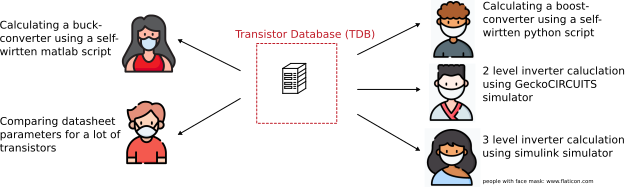
The key feature is the Python interface, to use the transistor data in self-written optimization routines.
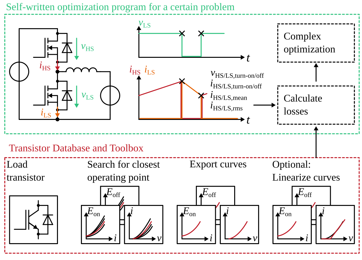
1. Python interface Use the transistor data in you self-written optimization program, see figure:
Automatic calculate your converter losses with many different transistors
Search the database for usable transistors for your application
Functions provided, to search for closest operating point
Functions provided, to linearize the transistor/diode conduction behaviour
Functions provided, to calculate the output capacitances Energy from the C_oss-curve
Use own loss measurements for above features (coming soon)
GUI
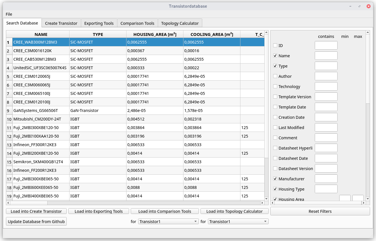
Manage, store and search the transistors
Export transistor models to programs like GeckoCIRCUITS, PLECS, Matlab/Octave
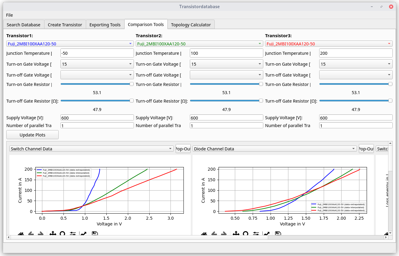
Compare transistors (interpolate switch loss data for new gate resistors and temperatures, …)
3 GUI Screenshots
3.1 Download and installation for windows
(For other operating systems, scroll down)
Download and install Git Installation file.
Download and install mongodb. Use the MongoDB community server, as platform, choose windows Link.
Download and run the transistordatabase here.
4 Why the transistordatabase?
When developing electronics, you need to calculate and simulate your schematic before building up the hardware. When it comes to the point of choosing a transistor, there is typically a lot of trouble with different programs. In typical cases, you use more than one program for your calculation, e.g. a self-written program for a first guess, and a schematic simulator to verify your results. Your colleague is working on another electronics topology, may using two other programs. Both of you have stored a few transistor-files on your computers. But due to other programs and another way of using them in a self-written program, your transistors will never be compatible with your colleagures program. If he want’s to use your transistors, he needs to generate them compleatly new from the datasheets to be compatible with his programs. Sharing programs and transistors will result in frustraction. This happens also in the same office (university / company / students).
The transistordatabase counteracts this problem. By a defined file format, you can handle these objects, export it to some propretery simulation software and share it by a .json-file to your colleagues or share it with the world by using the transistor database file exchange git repository.
4.1 Functionality overview
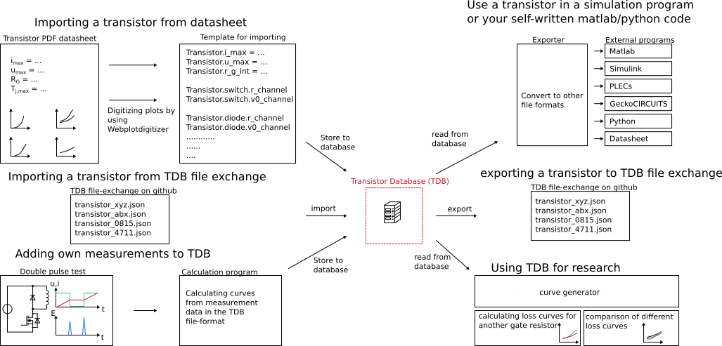
Functionality examples:
digitize transistor datasheet parameters and graphs and save it to the TDB
use this data for calculations in python (e.g. some loss calulations for a boost-converter)
export this data to matlab for calculations in matlab
export transistors to GeckoCIRCUITS simulation program
export transistors to Simulink simulation program
export transistors to PLECS simulation program
Note
Development status: Alpha
4.2 Complete documentation
The complete documentation can be found here.
5 Installation
5.1 Windows
5.1.1 Install Mongodb
For the first usage, you need to install mongodb. Install with standard settings. Use the MongoDB community server, as platform, choose windows Link.
5.1.2 Install git
Git Installation file. If you already have git installed, make sure you are using the latest version.
Note
During installation, you will be asked ‘Which editor would you like Git to use?’. Default is ‘Vim’, but it is one of the most complex one for beginners. Switch to ‘Notepad++’, ‘Nano’ or another one.
5.1.3 Install Python
Install latest Python version: Link.
5.1.4 Install Pycharm
5.1.5 Download and run executable
Download exe-file here:
5.2 Linux
Archlinux / Manjaro
Enable Arch-User-Repository (AUR).
sudo pacman -Syu mongodb-bin git pycharm
Ubuntu
sudo apt install python3 python3-pip git
Note
Install pycharm from Snapstore
5.3 All Operating systems: Install the transistor database
Inside pycharm, create a new project. Select ‘new environment using’ -> ‘Virtualenv’.
As a base interpreter, select ‘C:UsersxxxxxxAppDataLocalProgramsPythonPython39Python.exe’. Click on create.
Navigate to file -> settings -> Project -> Python Interpreter -> ‘+’ -> search for ‘transistordatabase’ -> ‘Install Package’
5.4 Complete minimal python example
Copy this example to a new pycharm project.
# load the python package
import transistordatabase as tdb

# update the database from the online git-repository
tdb.update_from_fileexchange()

# print the database
tdb.print_tdb()

# load a transistor from the database
transistor_loaded = tdb.load('CREE_C3M0016120K')

# export a virtual datasheet
transistor_loaded.export_datasheet()
On the output line, you should see a message which links to the datasheet file. Click on it to view the datasheet in your browser. If this works, you have set up the transistor database correctly.
6 transistordatabase’s usage
Import transistordatabase to your python program
import transistordatabase as tdb
6.1 Generate a new transistor
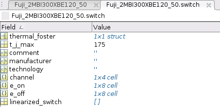
6.1.1 Transistor object basics
Transistor
|
+-Metadata
|
+-Switch
| +-Switch Metadata
| +-Channel Data
| +-Switching Data
|
+-Diode
| +-Diode Metadata
| +-Channel Data
| +-Switching Data
|
+-wp (temporary storage for further calculations)
6.1.2 Reading curves from the datasheet
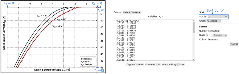
For reading datasheet curves, use the tool WebPlotDigitizer. There is a online-version available. Also you can download it for Linux, Mac and Windows. WebPlotDigitizer is open source software.
Channel data for switch and diode always needs to be positive. Some Manufacturers give diode data in the 3rd quadrant. Here is an example how to set the axes and export the data inside WebPlotDigitizer:
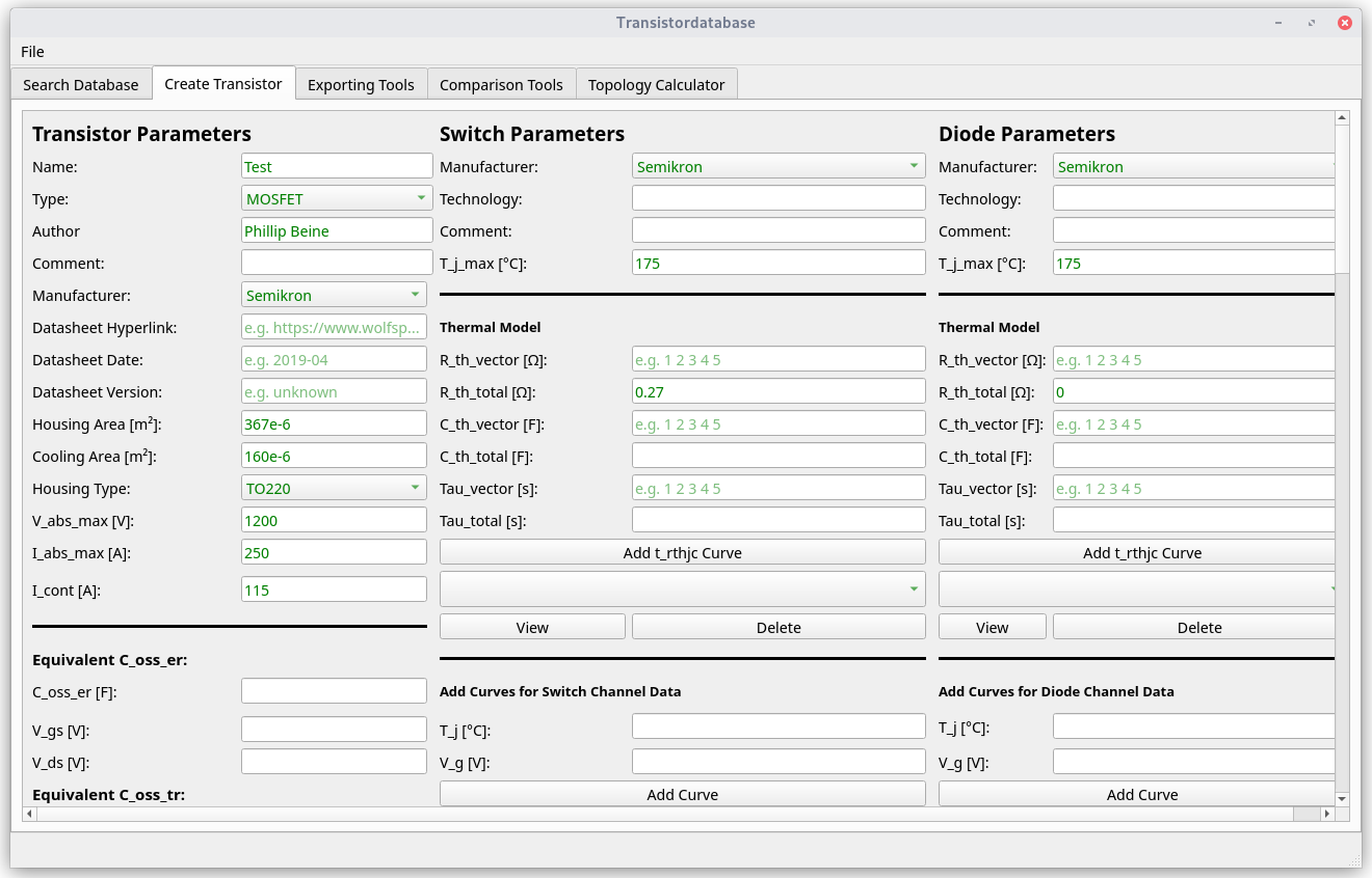
6.1.3 Use the template to generate a new transistor object
After digitizing the curves, you can use a template to generate a new transistor object and store it to the database. For this, see the template.
Some values need to follow some rules, e.g. due to different spelling versions, the manufacturers name or housing types must be written as in the lists below. Some general hints to fill the template:
In many cases, two capacity curves are specified in the data sheets. One curve for the full voltage range, and one with zoom to a small voltage range. To represent the stored curves in the best possible way, both curves can be read in and then merged.
c_rss_normal = csv2array('transistor_c_rss.csv', first_x_to_0=True)
c_rss_detail = csv2array('transistor_c_rss_detail.csv', first_x_to_0=True)

transistor_args = {
               ...
               'c_rss': {"t_j": 25, "graph_v_c": c_rss_merged},
                               ...
               }
6.3 Usage of Transistor.wp. in your programs
There is a subclass .wp where you can fill for further program calculations.
6.3.1 Full-automated example
Use the quickstart method to fill in the wp-class
There is a search function, that chooses the closes operating point. In the full-automated method, there are some predefined values
Chooses transistor.switch.t_j_max - 25°C as operating temperature to start search
Chooses transistor.i_abs_max/2 as operating current to start search
Chooses v_g = 15V as gate voltage to start search
transistor_loaded.quickstart_wp()
6.3.2 Half-automated example
Fill in the wp-class by a search-method to find the closes working point to your methods
Insert a working point of interest. The algorithm will find the closest working point and fills out the Transistor.wp.-class .. code-block:
transistor.update_wp(125, 15, 50)
6.3.3 Non-automated example
Fill in the wp-class manually
Look for all operating points manually. This will result in an error in case of no match. .. code-block:
transistor_loaded.wp.e_oss = transistor_loaded.calc_v_eoss()
transistor_loaded.wp.q_oss = transistor_loaded.calc_v_qoss()

# switch, linearize channel and search for losscurves
transistor_loaded.wp.switch_v_channel, transistor_loaded.wp.switch_r_channel = transistor_loaded.calc_lin_channel(25, 15, 150, 'switch')
transistor_loaded.wp.e_on = transistor_loaded.get_object_i_e('e_on', 25, 15, 600, 2.5).graph_i_e
transistor_loaded.wp.e_off = transistor_loaded.get_object_i_e('e_off', 25, -4, 600, 2.5).graph_i_e

# diode, linearize channel and search for losscurves
transistor_loaded.wp.diode_v_channel, transistor_loaded.wp.diode_r_channel = transistor_loaded.calc_lin_channel(25, -4, 150, 'diode')
6.4 Calculations with transistor objects
6.4.1 Parallel transistors
To parallel transistors use the function.
In case of no parameter paralleling is for 2 transistors
In case of parameter, paralleling is for x transistors. Example here is for three transistors.
transistor = load('Infineon_FF200R12KE3')
parallel_transistorobject = transistor.parallel_transistors(3)
After this, you can work with the transistor object as usual, e.g. fill in the .wp-workspace or export the device to Matlab, Simulink or GeckoCIRCUITS.
7 Export transistor objects
Using transistors within pyhton you have already seen. Now we want to take a closer look at exporting the transistors to other programs. These exporters are currently working. Some others are planned for the future.
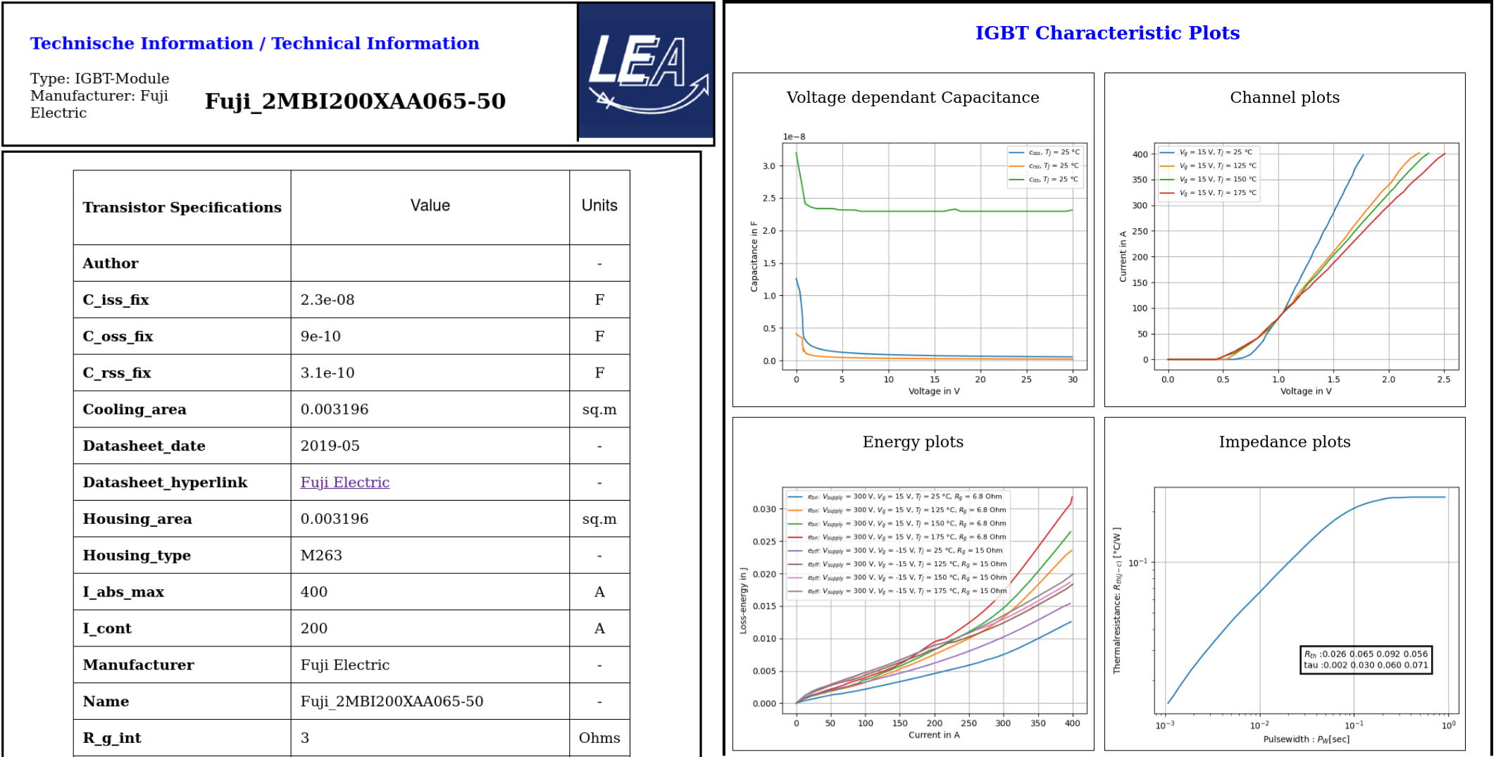
7.1 Export a Virtual datasheet
This function exports a virtual datasheet to see stored data in the database. Function display the output path of .html-file, which can be opened in your preferred browser.
transistor = tdb.load('Fuji_2MBI100XAA120-50')
transistor.export_datasheet()
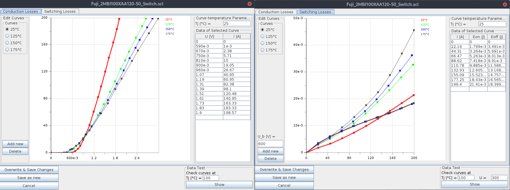
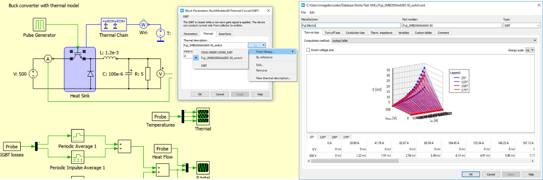
7.2 Export to GeckoCIRCUITS
GeckoCIRCUITS is an open source multi platform schematic simulator. Java required. Direct download link. At the moment you need to know the exporting parameters like gate resistor, gate-voltage and switching voltage. This will be simplified in the near future.
transistor = tdb.load('Fuji_2MBI100XAA120-50')
transistor.export_geckocircuits(600, 15, -4, 2.5, 2.5)
From now on, you can load the model into your GeckoCIRCUITS schematic.
Hint
It is also possible to control GeckoCIRCUITS from python, e.g. to sweep transistors. In this case, linux users should consider to run this Version of GeckoCIRCUITS instead the above one (port to OpenJDK).
7.3 Export to PLECS
For a thermal and loss simulation using PLECS simulation tool, it requires the transistor loss and characteristic curves to be loaded in XML(Version 1.1) file format. More information on how to load the XML data can be found from here. To export the transistor object from your database to plecs required xml file format, following lines need to be executed starting with loading the required datasheet.
transistor = tdb.load('Fuji_2MBI200XAA065-50')
transistor.export_plecs()
Outputs are xml files - one for switch and one for diode (if available), which can be then loaded into your schematic following the instructions as mentioned here. Note that if channel curves for the default gate-voltage are found missing then the xml files could not be possible to generate and a respective warning message is issued to the user. The user can change the default gate-voltage and switching voltage by providing an extra list argument as follows:
transistor = tdb.load('Fuji_2MBI200XAA065-50')
transistor.export_plecs([15, -15, 15, 0])
Note that all the four parameters (Vg_on, Vg_off) for IGBTs/Mosfets and (Vd_on, Vd_off) for reverse/body diodes are necessary to select the required curves that needs to be exported to switch and diode XMLs respectively.
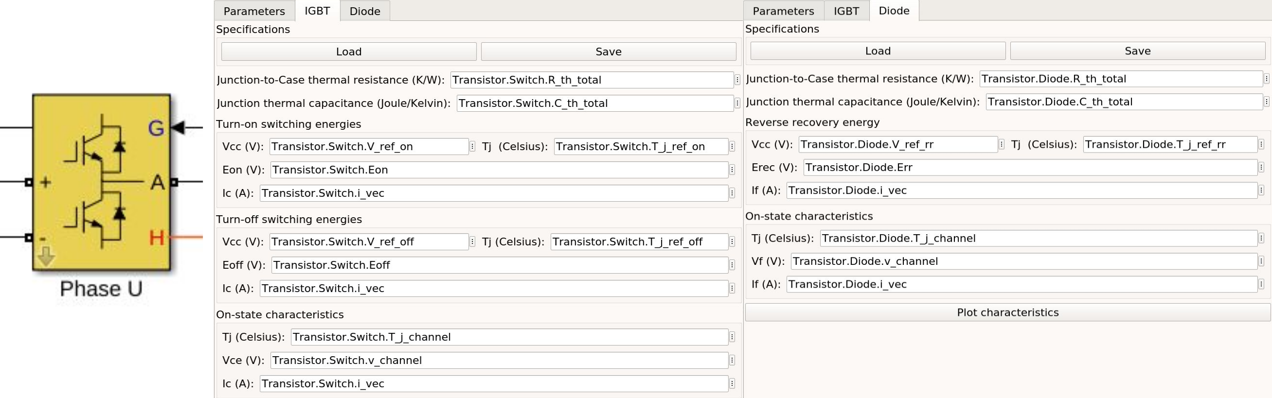
7.4 Export to Simulink
For a loss simulation in simulink, there is a IGBT model available, which can be found in this simulink model . Copy the model to you schematic and fill the parameters as shown in the figure. Export a transistor object from your database by using the following command. Example for a Infineon transistor. .. code-block:
transistor = tdb.load('Infineon_FF200R12KE3')
transistor.export_simulink_loss_model()
Output is a .mat-file, you can load in your matlab program to simulate. Now, you are able to sweep transistors within your simulation. E.g. some matlab-code:
load Infineon_FF200R12KE3_Simulink_lossmodel.mat;
load Infineon_FF300R12KE3_Simulink_lossmodel.mat;
load Fuji_2MBI200XBE120-50_Simulink_lossmodel.mat;
load Fuji_2MBI300XBE120-50_Simulink_lossmodel.mat;
Transistor_array = [Infineon_FF200R12KE3 Infineon_FF300R12KE3 Fuji_2MBI200XBE120-50 Fuji_2MBI300XBE120-50];
for i_Transistor = 1:length(Transistor_array)
    Transistor = Transistor_array(i_Transistor);
    out = sim('YourSimulinkSimulationHere');
7.5 Export to Matlab/Octave
Python dictionary can be exported to Matlab, see the following example:
transistor = tdb.load('Fuji_2MBI100XAA120-50')
transistor.export_matlab()
A .mat-file is generated, the exporting path will be displayed in the python console. You can load this file into matlab or octave.
8 Others
8.1 Roadmap
Planned features in 2022
Focus on adding self-measured data to the database
Working with self-measured data in exporters
Usability improvements
Stable software
8.2 Organisation
8.2.1 Bug Reports
Please use the issues report button within github to report bugs.
8.2.2 Changelog
Find the changelog here.
8.2.3 Contributing
Pull requests are welcome. For major changes, please open an issue first to discuss what you would like to change. For contributing, please refer to this section.
8.3 About
8.3.1 History and project status
This project started in 2020 as a side project and was initially written in matlab. It quickly became clear that the project was no longer a side project. The project should be completely rewritten, because many new complex levels have been added. To place the project in the open source world, the programming language python is used.
In January 2021 a very early alpha status was reached. First pip package was provided in may 2021. First GUI is provided in June 2022.
8.3.2 License
Licensed under GPLv3