Single Inverter Current Control
In this example a three phase inverter is supplying a load (rl1) via a filter (lc1) like shown in the figure below. From that model a FMU is built to create the environment.
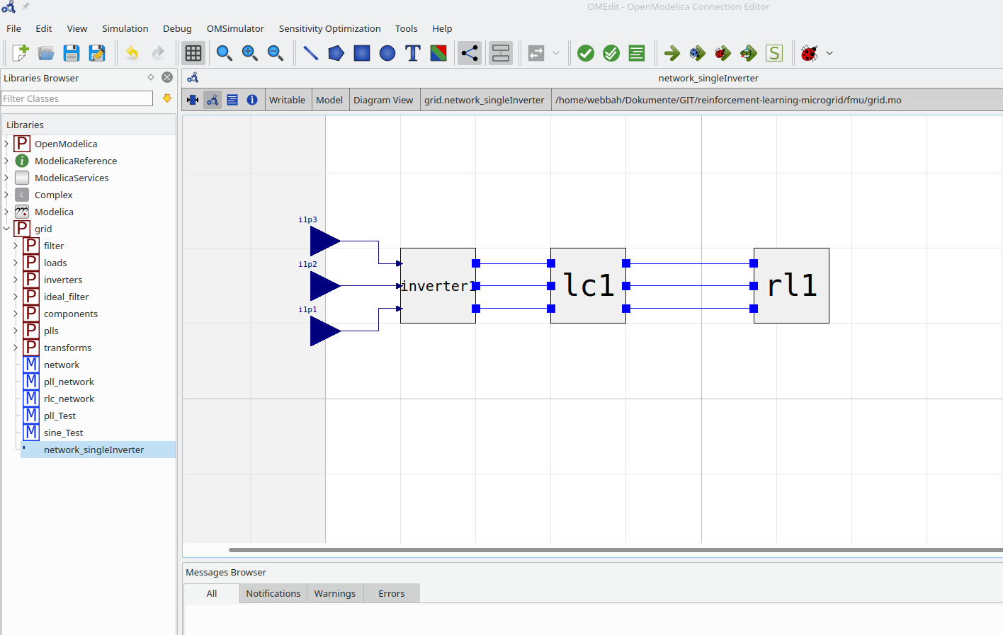
An optimization method developed by Berkenkamp et al. called Safe Controller Optimization (safeopt) is used which takes a Gaussian process and Bayesian optimization to safely determine “optimal” controller parameters. The goal of the standard PI current controller is to supply an exemplary 15 A d-current to the load.
The generated FMU is used in the environment to build up a gym env like the examples from OpenAI Gym (https://gym.openai.com/). The gym enviroment is defined in (examples/single_inverter_current_control_safe_opt.py). It generates a gym environment using
a reward function,
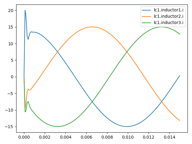
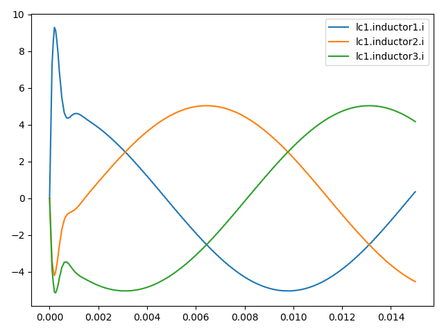
plotting the inductor values (current) from the lc1-filter (which should be controlled) like shown in the figure below,
simulating 300 timesteps of delta_t of the FMU grid.network_singleInverter.fmu (generated from the model in the plot above),
using the setpoints for the inverters (modulation indices) i1p{1,2,3} as inputs,
and the inductor currents and capacitor voltages of lc1-filter as outputs.
The agent used in this simple RL-example is taken from the class
SafeOptAgent. It contains the controller a
MultiPhaseDQCurrentSourcingController, which consists of multiphase
(3) PI controllers to control the current across the inductor of the
lc1-filter. There are also droop controllers implemented to calculate
e.g. the frequency drop due to load changes. The agent’s task is to find better
parameters for the current controllers (Kp & Ki). Therefore, they are
defined as mutable_params (e.g.
examples/single_inverter_current_control_safe_opt.py) to
adopt them between the episodes. The SafeOpt algorithm uses a Gaussian
process to estimate the performance of the controller. Thus, the
bounds and the lengthscale (c.f. examples/single_inverter_current_control_safe_opt.py) for
the gain parameters (Kp and Ki) have to be defined.
One can adjust one of the parameters (Kp or Ki) (1D case) or both of them (2D case) using the algorithm. Therefore, the following flag parameters have to be adjusted accoridngly:
To adjust only Kp set
adjust = 'Kp'To adjust only Ki set
adjust = 'Kp'To adjust only Kp and Ki set
adjust = 'Kpi'
Due to SafeOpt the agent need a safe starting point (Kp and Ki). Then it tries to calculate safely parameters with better performance. The performance is calculated using the reward function from the environment. There the mean-root-error (RME) from the measured currents and the setpoints are calculated. Additionally a barrier function is used to penalize over-currents. The barrier function can be adjusted using the parameter mu.
The safe threshold for the agent is set as safe_threshold-times of the initial performance (c.f. agents/safeopt.py). For example, safe_threshold = 1.2 and the initial reward is -10 the safe threshold would be -12.
In the end of the script a Runner is used to execute 10 episodes
using the agent to control the environment. For every episode the
controlled currents and the performance function as a function of Kp
and/or Ki are plotted.
Some exemplary results are shown below:
If
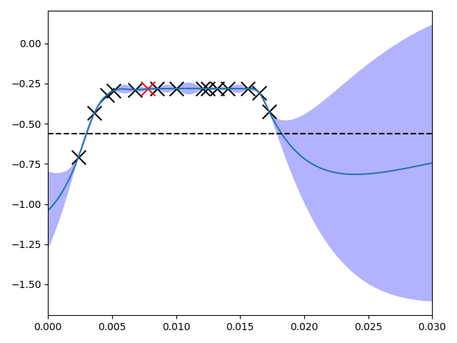
adjust == 'Kp', the agent tries to find an optimal value for the proportional gain (Kp) of the controller in the range of [0, 0.03] with a lengthscale of 0.01. In the figure below on the x-axis is the value for Kp and on the y-axis the performance value calculated using the reward function mentioned above.
If
adjust == 'Ki', the agent tries to find an optimal value for the integral gain (Ki) of the controller in the range of [0, 300] with a lengthscale of 50. In the figure below on the x-axis is the value for Ki and on the y-axis the performance value calculated using the reward function mentioned above.
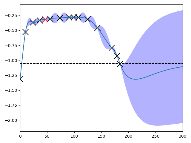
The - due to the algorithm - “unsafe” point on the right (for Kp as well as for Ki) is not due to overcurrent but due to bad performance due to permanent control error. The resulting currents for Kp = 0.01 and Ki = 0 (“unsafe” point on the right in the figure above) is shown in the picture below. Due to the high error compared to the reference value (15 A d-current), the performance is as bad as the algorithm defines it as unsafe - in comparison to the performance reached using the initial controller parameters.
If
adjust == 'Kpi', the agent tries to find an optimal value for the proportional gain (Kp) as well as for the integral gain (Ki) of the controller in the ranges of [0, 0.03] and a lengthscale of 0.01 for Kp and a range of [0, 300] and a lengthscale of 50 for Ki. In the figure below on the x-axis is the value for Kp, the y-axis the value for Ki and the z-axis the performance value calculated using the reward function.
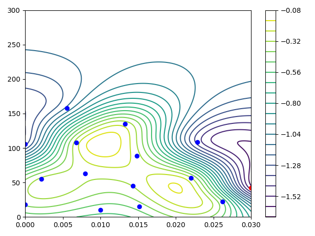
The results of the algorithm are printed into the console in the form like below:
Iteration, performance J, Params [Kp, Ki]
       J                                      Params
0  -0.527522                                [0.01, 10.0]
1  -0.442648    [0.01517286546392185, 14.85163114970222]
2  -0.318154    [0.01426989823624961, 44.96747682456248]
3  -0.296940   [0.007935547159879385, 63.12800825929393]
4  -0.286636    [0.01482713453607815, 88.70170996759624]
5  -0.286815  [0.006770598304777539, 108.12303673537075]
6  -0.280167  [0.013261084415467694, 135.24448051372738]
7  -0.313204   [0.02201710533671064, 56.446583269542394]
8  -1.387003  [0.022868977920736434, 108.40140778199653]
9  -0.304403   [0.002145673177669012, 55.14569829606201]
10 -0.480421   [0.026197353734745858, 22.29566509028389]
11 -1.097157  [0.0055262530542335535, 157.4879776902759]
12 -0.391706                    [0.0, 17.86728037560901]
13 -1.307038                    [0.0, 106.0724160092763]
14 -1.561142                    [0.03, 42.1020413015999]
The best performance in this short example of -0.280167 produces the parameter set of Kp = 0.0132… and Ki = 135.244…